The Predator-Prey Equation in Matlab_unable to meet integration tolerances without redu-CSDN博客

转载自：http://www-users.math.umd.edu/~jmr/246/predprey.html

The Predator-Prey Equation

Original Lotka-Volterra Model

We assume we have two species, herbivores with population x, and predators with propulation y. We assume that x grows exponentially in the absence of predators, and that y decays exponentially in the absence of prey. Consider, say, the system

Critical points:

syms x
 y

vars = [x, y];
eqs = [x*(1-y/2), y*(-1+x/2)];
[xc, yc] = solve(eqs(1), eqs(2));
[xc, yc]
A = jacobian(eqs, vars);
disp('Matrix of linearized system:'
)
subs(A, vars, [xc(1), yc(1)])
disp('eigenvalues:'
)
eig(ans)
disp('Matrix of linearized system:'
)
subs(A, vars, [xc(2), yc(2)])
disp('eigenvalues:'
)
eig(double(ans))

 
ans =
 
[ 0, 0]
[ 2, 2]
 
 
Matrix of linearized system:
 
ans =
 
[  1,  0]
[  0, -1]
 
 
eigenvalues:
 
ans =
 
  1
 -1
 
 
Matrix of linearized system:
 
ans =
 
[  0, -1]
[  1,  0]
 
 
eigenvalues:

ans =

        0 + 1.0000i
        0 - 1.0000i

Thus we have a center at (2, 2) and a saddle point at (0, 0), at least for the linearized system. This suggests the possibility of periodic orbits centered around (2, 2).

Phase Plot

rhs1 = @(t, x) ...

    [x(1)*(1-.5*x(2)); x(2)*(-1+.5*x(1))];
options = odeset('RelTol'
, 1e-6);
figure, hold on

for
 x0 = 0:.2:2
    [t, x] = ode45(rhs1, [0, 10], [x0;2]);
    plot(x(:,1), x(:,2))
end
, hold off

Plot of Populations vs. Time

We color-code the plots so you can see which ones go together.

colors = 'rgbyc'
;
figure, hold on

for
 x0 = 0:10
    [t, x] = ode45(rhs1, [0, 25], [x0/5; 2], options);
    subplot(2, 1, 1), hold on

    plot(t, x(:,1), colors(mod(x0,5)+1))
    subplot(2, 1, 2), hold on

    plot(t, x(:, 2), colors(mod(x0,5)+1))
    hold on

end

subplot(2, 1, 1)
xlabel t

ylabel 'x = prey'

subplot(2, 1, 2)
xlabel t

ylabel 'y = predators'

hold off

Modified Model with "Limits to Growth" for Prey (in Absence of Predators)

In the original equation, the population of prey increases indefinitely in the absence of predators. This is unrealistic, since they will eventually run out of food, so let's add another term limiting growth and change the system to

Critical points:

syms x
 y

vars = [x, y];
eqs = [x*(1-y/2-x/4), y*(-1+x/2)];
[xc, yc] = solve(eqs(1), eqs(2));
[xc, yc]
A = jacobian(eqs, vars);
disp('Matrix of linearized system:'
)
subs(A, vars, [xc(1), yc(1)])
disp('eigenvalues:'
)
eig(ans)
disp('Matrix of linearized system:'
)
subs(A, vars, [xc(2), yc(2)])
disp('eigenvalues:'
)
eig(ans)
disp('Matrix of linearized system:'
)
subs(A, vars, [xc(3), yc(3)])
disp('eigenvalues:'
)
eig(double(ans))

 
ans =
 
[ 0, 0]
[ 4, 0]
[ 2, 1]
 
 
Matrix of linearized system:
 
ans =
 
[  1,  0]
[  0, -1]
 
 
eigenvalues:
 
ans =
 
  1
 -1
 
 
Matrix of linearized system:
 
ans =
 
[ -1, -2]
[  0,  1]
 
 
eigenvalues:
 
ans =
 
 -1
  1
 
 
Matrix of linearized system:
 
ans =
 
[ -1/2,   -1]
[  1/2,    0]
 
 
eigenvalues:

ans =

  -0.2500 + 0.6614i
  -0.2500 - 0.6614i

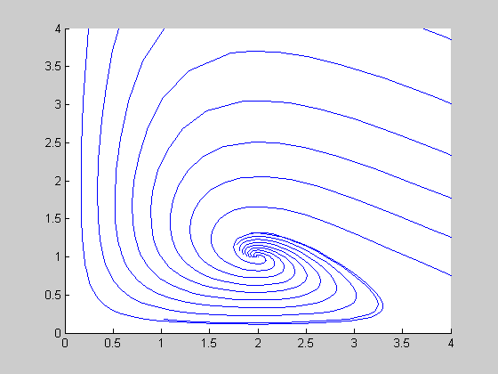
Thus we have saddles at (0, 0), (4, 0) and a stable spiral point at (2, 1).

rhs2 = @(t, x) ...

    [x(1)*(1-.5*x(2)-0.25*x(1)); x(2)*(-1+.5*x(1))];
figure, hold on

for
 x0 = 0:.2:2
    [t, x] = ode45(rhs2, [0, 10], [x0;1]);
    plot(x(:,1), x(:,2))
end

for
 x0 = 0:.2:2
    [t, x] = ode45(rhs2, [0, -10], [x0;1]);
    plot(x(:,1), x(:,2))
end

axis([0, 4, 0, 4]), hold off

Warning: Failure at t=-3.380660e+000.  Unable to meet integration tolerances without reducing the step size below the smallest value allowed (7.105427e-015) at time t.
Warning: Failure at t=-3.535072e+000.  Unable to meet integration tolerances without reducing the step size below the smallest value allowed (7.105427e-015) at time t.
Warning: Failure at t=-3.735844e+000.  Unable to meet integration tolerances without reducing the step size below the smallest value allowed (7.105427e-015) at time t.
Warning: Failure at t=-3.984664e+000.  Unable to meet integration tolerances without reducing the step size below the smallest value allowed (7.105427e-015) at time t.
Warning: Failure at t=-4.299922e+000.  Unable to meet integration tolerances without reducing the step size below the smallest value allowed (1.421085e-014) at time t.
Warning: Failure at t=-4.719481e+000.  Unable to meet integration tolerances without reducing the step size below the smallest value allowed (1.421085e-014) at time t.
Warning: Failure at t=-5.332082e+000.  Unable to meet integration tolerances without reducing the step size below the smallest value allowed (1.421085e-014) at time t.
Warning: Failure at t=-6.437607e+000.  Unable to meet integration tolerances without reducing the step size below the smallest value allowed (1.421085e-014) at time t.

Plot of Populations vs. Time

figure, hold on

for
 x0 = 0:20
    [t, x] = ode45(rhs2, [0, 25], [x0/5; 1], options);
    subplot(2, 1, 1), hold on

    plot(t, x(:,1), colors(mod(x0,5)+1))
    subplot(2, 1, 2), hold on

    plot(t, x(:, 2), colors(mod(x0,5)+1))
    hold on

end

subplot(2, 1, 1)
xlabel t

ylabel 'x = prey'

subplot(2, 1, 2)
xlabel t

ylabel 'y = predators'

hold off