2.深度学习练习：Logistic Regression with a Neural Network mindset

本文节选自吴恩达老师《深度学习专项课程》编程作业，在此表示感谢。

课程链接：https://www.deeplearning.ai/deep-learning-specialization/

You will learn to:

• Build the general architecture of a learning algorithm, including:
  • Initializing parameters
  • Calculating the cost function and its gradient
  • Using an optimization algorithm (gradient descent)
• Gather all three functions above into a main model function, in the right order.

你将会学到深度学习的通用结构，包括：

• 参数初始化
• 计算损失函数和梯度
• 使用优化算法（梯度下降）

---

目录

1 - Packages

2 - Overview of the Problem set

3 - General Architecture of the learning algorithm（掌握）

4 - Building the parts of our algorithm

4.1 - Helper functions

4.2 - Initializing parameters

4.3 - Forward and Backward propagation（掌握）

4.4 - Optimization

4.5 - Predict

5 - Merge all functions into a model

---

1 - Packages

First, let's run the cell below to import all the packages that you will need during this assignment.

• numpy is the fundamental package for scientific computing with Python.
• h5py is a common package to interact with a dataset that is stored on an H5 file.
• matplotlib is a famous library to plot graphs in Python.
• PIL and scipy are used here to test your model with your own picture at the end.

import numpy as np
import matplotlib.pyplot as plt
import h5py
import scipy
from PIL import Image
from scipy import ndimage
from lr_utils import load_dataset  # 这个函数在文件夹下的 py 文件中

%matplotlib inline

---

2 - Overview of the Problem set

Problem Statement: You are given a dataset ("data.h5") containing:

- a training set of m_train images labeled as cat (y=1) or non-cat (y=0)
- a test set of m_test images labeled as cat or non-cat
- each image is of shape (num_px, num_px, 3) where 3 is for the 3 channels (RGB). Thus, each image is square (height = num_px) and (width = num_px).

每一张图片的shape:(num_px, num_px, 3)，3代表3个通道（RGB）。

You will build a simple image-recognition algorithm that can correctly classify pictures as cat or non-cat.

Let's get more familiar with the dataset. Load the data by running the following code.

Many software bugs in deep learning come from having matrix/vector dimensions that don't fit. If you can keep your matrix/vector dimensions straight you will go a long way toward eliminating many bugs.

Exercise: Find the values for:

- m_train (number of training examples)
- m_test (number of test examples)
- num_px (= height = width of a training image)

Remember that train_set_x_orig is a numpy-array of shape (m_train, num_px, num_px, 3). For instance, you can access m_train by writing train_set_x_orig.shape[0].

m_train = train_set_x_orig.shape[0]
m_test = test_set_x_orig.shape[0]
num_px = train_set_x_orig.shape[1]

For convenience, you should now reshape images of shape (num_px, num_px, 3) in a numpy-array of shape (num_px ∗∗ num_px ∗∗ 3, 1). After this, our training (and test) dataset is a numpy-array where each column represents a flattened image. There should be m_train (respectively m_test) columns.

Exercise: Reshape the training and test data sets so that images of size (num_px, num_px, 3) are flattened into single vectors of shape (num_px ∗∗ num_px ∗∗ 3, 1).

A trick when you want to flatten a matrix X of shape (a,b,c,d) to a matrix X_flatten of shape (b∗∗c∗∗d, a) is to use:

X_flatten = X.reshape(X.shape[0], -1).T      # X.T is the transpose of X

train_set_x_flatten = train_set_x_orig.reshape(train_set_x_orig.shape[0], -1).T
test_set_x_flatten  = test_set_x_orig.reshape(test_set_x_orig.shape[0], -1).T

Let's standardize our dataset.

train_set_x = train_set_x_flatten/255.
test_set_x = test_set_x_flatten/255.

**What you need to remember:**

Common steps for pre-processing a new dataset are:

• Figure out the dimensions and shapes of the problem (m_train, m_test, num_px, ...)
• Reshape the datasets such that each example is now a vector of size (num_px * num_px * 3, 1)
• "Standardize" the data

新数据集常用的预处理顺序是：

• 查看训练集、测试集大小和样本的形状（m_train，m_test，num_px等）
• 重塑数据集，使每个样本变成为一个大小为(num_px * num_px * 3, 1)的向量
• 数据“标准化”处理

---

3 - General Architecture of the learning algorithm（掌握）

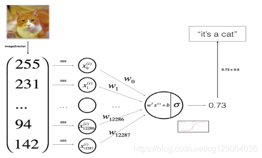
You will build a Logistic Regression, using a Neural Network mindset. The following Figure explains why Logistic Regression is actually a very simple Neural Network!

Mathematical expression of the algorithm:

For one example ：

                                                                                                                         

                                ​​​​​​​        ​​​​​​​        ​​​​​​​        ​​​​​​​        ​​​​​​​        ​​​​​​​        ​​​​​​​        ​​​​​​​        ​​​​​​​        ​​​​​​​        

                                                                                                 ​

The cost is then computed by summing over all training examples:

Key steps: In this exercise, you will carry out the following steps:

• - Initialize the parameters of the model
• - Learn the parameters for the model by minimizing the cost  
• - Use the learned parameters to make predictions (on the test set)
• - Analyse the results and conclude

关键步骤：在这个练习中，你将会进行以下步骤：

• 初始化模型参数
• 通过降低损失来学习模型参数
• 使用学习到的参数来预测（在测试集上预测）
• 分析预测结果和总结

---

4 - Building the parts of our algorithm

The main steps for building a Neural Network are:

1. Define the model structure (such as number of input features)
2. Initialize the model's parameters
3. Loop:
   • Calculate current loss (forward propagation)
   • Calculate current gradient (backward propagation)
   • Update parameters (gradient descent)

You often build 1-3 separately and integrate them into one function we call model().

4.1 - Helper functions

Exercise: Using your code from "Python Basics", implement sigmoid()

def sigmoid(z):
    """
    Compute the sigmoid of z

    Arguments:
    z -- A scalar or numpy array of any size.

    Return:
    s -- sigmoid(z)
    """

    s = 1 / (1 + np.exp(-z))
   
    return s

4.2 - Initializing parameters

def initialize_with_zeros(dim):
    """
    This function creates a vector of zeros of shape (dim, 1) for w and initializes b to 0.
    
    Argument:
    dim -- size of the w vector we want (or number of parameters in this case)
    
    Returns:
    w -- initialized vector of shape (dim, 1)
    b -- initialized scalar (corresponds to the bias)
    """
    
   
    w = np.zeros((dim, 1))
    b = 0

    assert(w.shape == (dim, 1))
    assert(isinstance(b, float) or isinstance(b, int))
    
    return w, b

4.3 - Forward and Backward propagation（掌握）

Now that your parameters are initialized, you can do the "forward" and "backward" propagation steps for learning the parameters.

Exercise: Implement a function propagate() that computes the cost function and its gradient.

Hints:

Forward Propagation:

• You get X
• You compute

•  You calculate the cost function:

Here are the two formulas you will be using:   

# GRADED FUNCTION: propagate

def propagate(w, b, X, Y):
    """
    Implement the cost function and its gradient for the propagation explained above

    Arguments:
    w -- weights, a numpy array of size (num_px * num_px * 3, 1)
    b -- bias, a scalar
    X -- data of size (num_px * num_px * 3, number of examples)
    Y -- true "label" vector (containing 0 if non-cat, 1 if cat) of size (1, number of examples)

    Return:
    cost -- negative log-likelihood cost for logistic regression
    dw -- gradient of the loss with respect to w, thus same shape as w
    db -- gradient of the loss with respect to b, thus same shape as b
    
    Tips:
    - Write your code step by step for the propagation. np.log(), np.dot()
    """
    
    m = X.shape[1]
    
    # FORWARD PROPAGATION (FROM X TO COST)
   
    A = sigmoid(np.dot(w.T, X) + b)
    cost = -1/m * np.sum(Y*np.log(A) + (1-Y)*np.log(1-A))
    
    # BACKWARD PROPAGATION (TO FIND GRAD)
 
    dw = 1/m * np.dot(X, (A-Y).T)
    db = 1/m * np.sum(A-Y)


    assert(dw.shape == w.shape)
    assert(db.dtype == float)
    cost = np.squeeze(cost)
    assert(cost.shape == ())
    
    grads = {"dw": dw,
             "db": db}
    
    return grads, cost

4.4 - Optimization

Exercise: Write down the optimization function. The goal is to learn  and  by minimizing the cost function . For a parameter , the update rule is  where  is the learning rate.

def optimize(w, b, X, Y, num_iterations, learning_rate, print_cost = False):
    """
    This function optimizes w and b by running a gradient descent algorithm
    
    Arguments:
    w -- weights, a numpy array of size (num_px * num_px * 3, 1)
    b -- bias, a scalar
    X -- data of shape (num_px * num_px * 3, number of examples)
    Y -- true "label" vector (containing 0 if non-cat, 1 if cat), of shape (1, number of examples)
    num_iterations -- number of iterations of the optimization loop
    learning_rate -- learning rate of the gradient descent update rule
    print_cost -- True to print the loss every 100 steps
    
    Returns:
    params -- dictionary containing the weights w and bias b
    grads -- dictionary containing the gradients of the weights and bias with respect to the cost function
    costs -- list of all the costs computed during the optimization, this will be used to plot the learning curve.
    
    Tips:
    You basically need to write down two steps and iterate through them:
        1) Calculate the cost and the gradient for the current parameters. Use propagate().
        2) Update the parameters using gradient descent rule for w and b.
    """
    
    costs = []
    
    for i in range(num_iterations):
        
        
        # Cost and gradient calculation (≈ 1-4 lines of code)
        grads, cost = propagate(w, b, X, Y)
 
        
        # Retrieve derivatives from grads
        dw = grads["dw"]
        db = grads["db"]
        
        # update rule (≈ 2 lines of code)
       
        w = w - learning_rate * dw
        b = b - learning_rate * db
        
        # Record the costs
        if i % 100 == 0:
            costs.append(cost)
        
        # Print the cost every 100 training examples
        if print_cost and i % 100 == 0:
            print ("Cost after iteration %i: %f" %(i, cost))
    
    params = {"w": w,
              "b": b}
    
    grads = {"dw": dw,
             "db": db}
    
    return params, grads, costs

4.5 - Predict

Exercise: The previous function will output the learned w and b. We are able to use w and b to predict the labels for a dataset X. Implement the predict() function. There is two steps to computing predictions:

1.Calculate 

2. Convert the entries of a into 0 (if activation <= 0.5) or 1 (if activation > 0.5), stores the predictions in a vector `Y_prediction`. If you wish, you can use an `if`/`else` statement in a `for` loop (though there is also a way to vectorize this). 

def predict(w, b, X):
    '''
    Predict whether the label is 0 or 1 using learned logistic regression parameters (w, b)
    
    Arguments:
    w -- weights, a numpy array of size (num_px * num_px * 3, 1)
    b -- bias, a scalar
    X -- data of size (num_px * num_px * 3, number of examples)
    
    Returns:
    Y_prediction -- a numpy array (vector) containing all predictions (0/1) for the examples in X
    '''
    
    m = X.shape[1]
    Y_prediction = np.zeros((1,m))
    w = w.reshape(X.shape[0], 1)
    
    # Compute vector "A" predicting the probabilities of a cat being present in the picture
    
    A = sigmoid(np.dot(w.T, X) + b)

    for i in range(A.shape[1]):
        
        # Convert probabilities A[0,i] to actual predictions p[0,i]
        if A[0,i] > 0.5:
            Y_prediction[0, i] = 1 
        else: 
            Y_prediction[0, i] = 0

    
    assert(Y_prediction.shape == (1, m))
    
    return Y_prediction

**What to remember:** You've implemented several functions that:

- Initialize (w,b)

- Optimize the loss iteratively to learn parameters (w,b):

- computing the cost and its gradient

- updating the parameters using gradient descent

- Use the learned (w,b) to predict the labels for a given set of examples

需要记住的，你已经实现了一些函数：

• 初始化（w,b）
• 迭代优化损失来学习参数（w,b）
• 计算损失和其梯度
• 使用梯度下降来更新参数
• 使用学习到的参数来预测给定样本的标签值

---

5 - Merge all functions into a model

You will now see how the overall model is structured by putting together all the building blocks (functions implemented in the previous parts) together, in the right order.

Exercise: Implement the model function. Use the following notation:

- Y_prediction for your predictions on the test set
- Y_prediction_train for your predictions on the train set
- w, costs, grads for the outputs of optimize()

def model(X_train, Y_train, X_test, Y_test, num_iterations = 2000, learning_rate = 0.5, print_cost = False):
   
 """
    Builds the logistic regression model by calling the function you've implemented previously
    
    Arguments:
    X_train -- training set represented by a numpy array of shape (num_px * num_px * 3, m_train)
    Y_train -- training labels represented by a numpy array (vector) of shape (1, m_train)
    X_test -- test set represented by a numpy array of shape (num_px * num_px * 3, m_test)
    Y_test -- test labels represented by a numpy array (vector) of shape (1, m_test)
    num_iterations -- hyperparameter representing the number of iterations to optimize the parameters
    learning_rate -- hyperparameter representing the learning rate used in the update rule of optimize()
    print_cost -- Set to true to print the cost every 100 iterations
    
    Returns:
    d -- dictionary containing information about the model.
    """
    
  
    # initialize parameters with zeros (≈ 1 line of code)
   
    w, b = initialize_with_zeros(X_train.shape[0])
   
    # Gradient descent (≈ 1 line of code)
   
    parameters, grads, costs = optimize(w, b, X_train, Y_train, num_iterations, learning_rate, print_cost)
   
    # Retrieve parameters w and b from dictionary "parameters"
    w = parameters["w"]
    b = parameters["b"]
    
    # Predict test/train set examples (≈ 2 lines of code)
   
    Y_prediction_test = predict(w, b, X_test)
    Y_prediction_train = predict(w, b, X_train)
  
    # Print train/test Errors
    print("train accuracy: {} %".format(100 - np.mean(np.abs(Y_prediction_train - Y_train)) * 100))
    print("test accuracy: {} %".format(100 - np.mean(np.abs(Y_prediction_test - Y_test)) * 100))

    
    d = {"costs": costs,
         "Y_prediction_test": Y_prediction_test, 
         "Y_prediction_train" : Y_prediction_train, 
         "w" : w, 
         "b" : b,
         "learning_rate" : learning_rate,
         "num_iterations": num_iterations}
    
    return d


d = model(train_set_x, train_set_y, test_set_x, test_set_y, num_iterations = 2000, learning_rate = 0.005, print_cost = True)