浅析简单神经网络的基本原理与实现

最新推荐文章于 2024-03-15 16:07:03 发布

ChiLi-L

最新推荐文章于 2024-03-15 16:07:03 发布

阅读量8k

点赞数 4

分类专栏：深度学习

本文链接：https://blog.csdn.net/chichichich/article/details/80534455

版权

深度学习专栏收录该内容

5 篇文章 1 订阅

订阅专栏

最近在看Andrew Ng 老师的神经网络和深度学习课程视频，非常值得像我这样的新手看，因此我一边看视频，一边来总结一下，也算是对学习知识的一种巩固和理解的加深，如果有表达不当的地方，希望多多包涵。
前面一篇文章里介绍了逻辑回归，为什么会先介绍逻辑回归呢？其实是为了引出神经网络的，逻辑回归可以看作是仅含一个神经元的单层神经网络。在机器学习/CNN系列小问题（1）：逻辑回归和神经网络之间有什么关系？这篇博文里直观的介绍了两者之间的关系。
另外推荐一篇博文，很直观并且图文并茂的介绍了神经网络的基础知识，非常适合不知道什么是神经网络的人看，我这篇文章中的一些图片就是引用自这边博文，给出地址：神经网络浅讲：从神经元到深度学习（作者：计算机的潜意识）

浅层神经网络

逻辑回归是最简单的一种神经网络，它的网络图为：
逻辑回归的网络结构
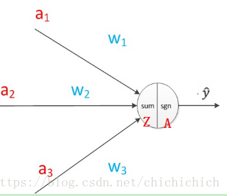
图中圆圈为神经元，假设输入为X，含有三个特征（a1, a2, a3）。为了直观的理解，可以认为完成了两个步骤：

线性计算： $Z^{[1]}=W^{[1]}X+b$
非线性计算： $A^{[1]}=\sigma(Z^{[1]})$
这里的上标 $^{[1]}$ 约定为网络的层次编号，在图中只有一个神经元即输出层，因此编号为1。图中A就是逻辑回归的输出。有了这个认识，我们再来看一下单隐层的神经网络。

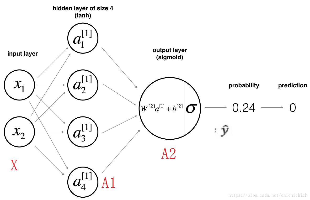
上图中，第一列圆圈代表输入层，第二列圆圈就是神经网络的中间层，这里的中间层只有一层，输出层与逻辑回归的输出层一致。在神经网络中，输入层是已知的，是用户输入的数据，因此不将输入层看出神经网络的网络层，因此上图的神经网络只包含一层隐藏层和一层输出层，又称为双层神经网络。同样，为了区分神经元在神经网络中的位置，我们分别用上标 $^{[l]}$ 和下标 $_i$ 代表神经网络所处的网络层次l和在该层中的位置i。如 $a^{[1]}_1$ 则是第一层的第一个神经元。
同样，单隐层中的神经元也包括了以上两个处理步骤，以此图为例， $X=\begin{bmatrix}x_1 \\ x_2 \end{bmatrix}=A^{[0]}$ 其流程为：
1.隐藏层：
线性计算： $Z^{[1]}=W^{[1]}X+b^{[1]}$
非线性计算： $A^{[1]}=g(Z^{[1]})$

2.输出层
线性计算： $Z^{[2]}=W^{[2]}A^{[1]}+b^{[2]}$
非线性计算： $A^{[2]}=\sigma(Z^{[2]})$

$A^{[2]}$ 就是此模型的输出预测值。
隐藏层中的g可以是任意的激活函数，例如ReLu函数，tanh函数,ELU函数，PReLu函数以及sigmoid函数，而输出层在二分类问题中经常采用sigmoid函数。

深层神经网络

神经神经网络就是在浅层神经网络的基础上增加了隐藏层的数量，即隐藏层的数量大于1.
约定用 L 代表神经网络的网络层数， $n^{[l]}$ 代表 $l$ 层中的神经元数量， $A^{[1]}$ 为每一层的输出。我们都采用向量化的表示方法来计算神经网络中每一步的结果，因此需要注意每一个向量的维度大小。给出以下五层的什么网络图：
深层神经网络
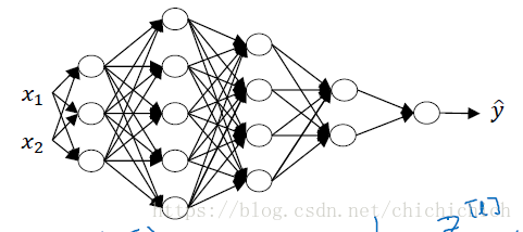
图中，输入有 $2$ 个属性，假设输入样本共有 m 个，则输入样本 X 的维度为 $(2,m)$ ， $n^{[1]}=3$ , $n^{[2]}=5$ , $n^{[3]}=4$ , $n^{[4]}=2$ , $n^{[5]}=1$ ，因此 $W^{[1]}$ 的维度为 $(3，2)$ , $W^{[2]}$ 的维度为 $(5，3)$ , $W^{[3]}$ 的维度为 $(4, 5)$ , $W^{[4]}$ 的维度为 $(2， 4)$ , $W^{[5]}$ 的维度为 $(1,2)$ 。

推广到一般，有：若输入有 $n_x$ 个属性，假设输入样本共有 m 个，则 X的维度为 $(n_x,m)$ ，而每层W 的维度为 $W^{[l]} : (n^{[l]}, n^{[l-1]})$ , A 和 b 的维度均为 $(n^{[l]}, m)$ 。
好，看完了神经网络从输入到输出的整个过程，我们怎么能够通过神经网络获得最优的参数 $W^{[l]}，b^{[l]}$ 呢？
还记得逻辑回归的参数优化过程吗？梯度下降法在神经网络的参数优化过程中也是至关重要的一部分。

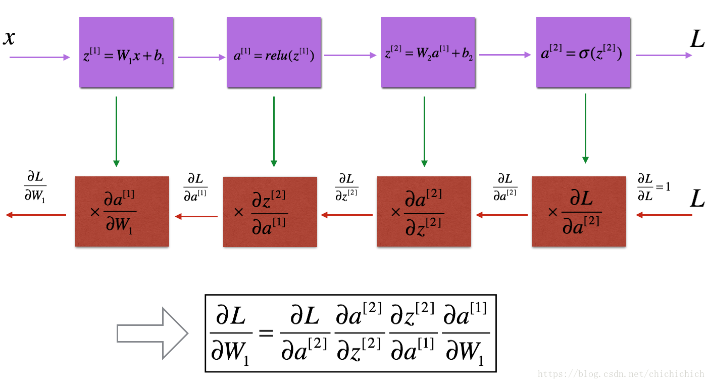
神经网络中的正向传播和反向传播的计算公式为：
前向和反向

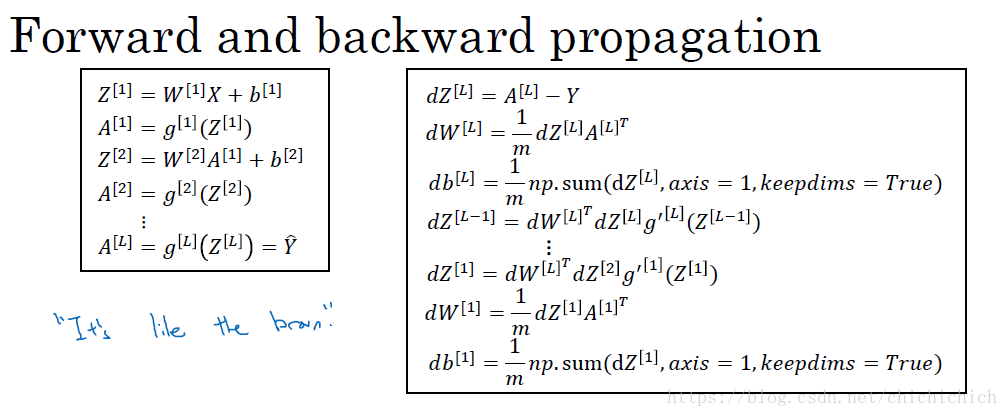
左边为我在上面给出来的正向传播的过程，右图则为反向传播（计算每个变量的梯度），在实际训练中，我们需要保存每一步的中间参数，保存为cache,如： $W^{[l]}，b^{[l]}，A^{[l]}, Z^{[l]}$ ，这些参数需要在反向传播中用来计算梯度，而 $dW^{[l]}，db^{[l]}$ 则用来计算梯度下降，梯度下降计算公式( $\alpha$ 是学习率)：

W [l] = W [l] - α * d W [l]

$W^{[l]} = W^{[l]} - \alpha*dW^{[l]}$

b [l] = b [l] - α * d b [l]

$b^{[l]} = b^{[l]} - \alpha*db^{[l]}$

这个过程画图表示，包括上面一部分的正向传播和下面一部分的反向传播，反向传播的输入为损失函数！
神经网络的梯度下降过程

因此可以根据下图的流程进行编程，搭建一个简单的神经网络。
程序流程

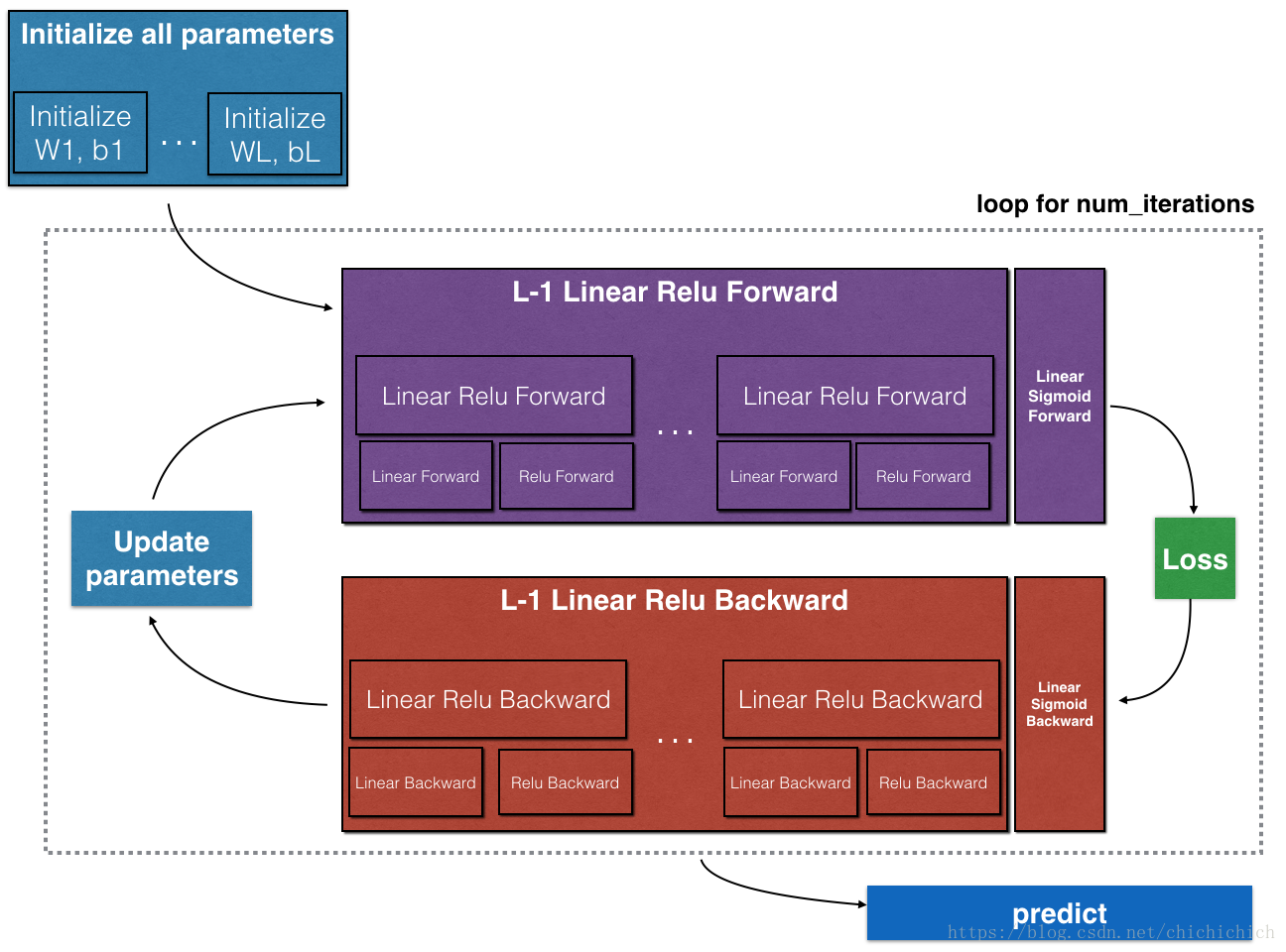
中间层为ReLu函数，输出层为sigmoid函数的神经网络伪实际上就是实现 [LINEAR -> RELU]*(L-1)次，LINEAR -> SIGMOID 1次。代码：

初始化代码和中间函数:

X=X_train #假设输入以及标准化，维度（nx,m）
Y=Y_train #实际训练样本的标签  维度(1,m)

#layers_dims的长度为网络层数，每个元素为整数，代表第i层的神经元数量设置网络结构，n_x为输入层，n_y为输出层，n_h(i)为隐藏层单元数
layers_dims = (n_x, n_h1,n_h2,..., n_y)  #n_h数量可以根据自己需要设置

#对每一层进行初始化
def initialize_parameters(layer_dims):
    np.random.seed(3)
    parameters = {}
    L = len(layer_dims)            # number of layers in the network
    # 根据上文给出的每一层的矩阵维度公式进行初始化，W初始化为数值很小的随机数，b初始化为0
    for l in range(1, L):
        parameters['W' + str(l)] = np.random.rand(layer_dims[l],layer_dims[l-1]) * 0.01
        parameters['b' + str(l)] = np.zeros((layer_dims[l],1))       
    return parameters

def linear_forward(A_prew, W, b):    #线性模型计算函数，求Z。这里的A其实是前一层的输出值
    Z = np.dot(W,A_prew) + b          #计算Z
    assert(Z.shape == (W.shape[0], A.shape[1]))    #保证矩阵维度正确
    cache = (A_prew, W, b)     #将变量保存下来，之后会用到   
    return Z, cache      

#通过正向传播计算Z和A，A_prev是前一层的输出，activation就是指定激活函数类型
def linear_activation_forward(A_prev, W, b, activation):
    if activation == "sigmoid":  #当激活函数为sigmoid函数
        Z, linear_cache = linear_forward(A_prev,W,b)  #调用线性模型求Z
        #调用sigmoid函数，这里的 activation_cache就是Z
        A, activation_cache = sigmoid(Z)   
    elif activation == "relu":
        # Inputs: "A_prev, W, b". Outputs: "A, activation_cache".
        Z, linear_cache = linear_forward(A_prev, W, b)  
        A, activation_cache = relu(Z) #activation_cache = Z
    assert (A.shape == (W.shape[0], A_prev.shape[1]))  #保证矩阵维度正确在神经网络中很重要
    cache = (linear_cache, activation_cache)  #输出缓存包括（[A_prew,W,b],[Z]）
    return A, cache

L层网络的正向传播实现：

# 实现L层神经网络的正向传播，输出最终结果AL，并保存中间变量caches。
def L_model_forward(X, parameters):
    caches = []
    A = X
    L = len(parameters) // 2                  # 网络层数量, [W,b]

    # 实现 [LINEAR -> RELU]*(L-1). Add "cache" to the "caches" list.
    for l in range(1, L):
        A_prev = A  #计算下一层的输出A，A_prew为A的前一层输出
        #调用linear_activation_forward 得到A，和中间变量
        A, cache = linear_activation_forward(A_prev,parameters['W' + str(l)], 
                                    parameters['b' + str(l)],activation='relu')        
        caches.append(cache)    #将每一层的中间变量保存到一个list里面

    # 实现最后一层输出层 LINEAR -> SIGMOID. Add "cache" to the "caches" list.
    AL, cache = linear_activation_forward(A ,parameters['W' + str(L)],
                                     parameters['b' + str(L)], activation='sigmoid')
    caches.append(cache)   
    assert(AL.shape == (1,X.shape[1]))            
    return AL, caches    # AL是整个网络一次正向传播的最终输出结果，caches保存了所有的中间变量

计算损失函数

#计算损失函数
def compute_cost(AL, Y):    
    m = Y.shape[1]
    # Compute loss from aL and y.，用损失函数公式计算，可以参考上一篇文章逻辑回归的损失函数公式
    cost = - np.sum(np.multiply(np.log(AL),Y) + np.multiply(np.log(1 - AL),(1 - Y)))/m   
    cost = np.squeeze(cost)     # 将cost转换成需要大小，如(将 [[17]] 变成 17)    
    return cost

L层网络的反向传播

# 计算梯度dA,dW,db的函数
def linear_activation_backward(dA, cache, activation):    
    linear_cache, activation_cache = cache   #linear_cache=[A_pre,w,b],activation_cache = z   
    A_prev, W, b = linear_cache  # 从正向传播的缓存中导出所需要的变量
     m = A_prev.shape[1]  #样本数量
    if activation == "relu":
        #调用relu函数的倒数公式计算dZ，这个只在反向传播的第一层用到
        dZ = relu_backward(dA, activation_cache)   

    elif activation == "sigmoid":
        # 调用sigmoid函数的梯度，这个只用到了一次，用在反向传播的第一层
        dZ = sigmoid_backward(dA, activation_cache)

    dW = np.dot(dZ,A_prev.T)/m    #  求W的梯度
    db = np.sum(dZ,axis=1 , keepdims=True)/m  #求b的梯度
    dA_prev = np.dot(W.T,dZ)   #求A的梯度，用于计算下一层网络的梯度

    return dA_prev, dW, db

# L层网络的反向传播，计算每层的梯度，保存到grads中
def L_model_backward(AL, Y, caches):
    grads = {}   #用来保存梯度值dA,dW,db
    L = len(caches) # the number of layers
    m = AL.shape[1]  #样本数量
    Y = Y.reshape(AL.shape) # after this line, Y is the same shape as AL
    # 初始化反向传播的输入值，dAL是损失函数的对AL求偏导数
    dAL = - np.divide(Y, AL) - np.divide((1- Y),(1-AL))

    # 第L层网络实现 (SIGMOID -> LINEAR) 的梯度. 得到dAL
    ### START CODE HERE ### (approx. 2 lines)
    current_cache = caches[L-1]   # 取L层的参数[dAL,dW,db],并且将这些值保存紧grads中
    grads["dA" + str(L)], grads["dW" + str(L)], grads["db" + str(L)] = linear_activation_backward(
                        dAL, current_cache, activation = "sigmoid")

    #实现前L-1层的梯度，保存到grads中
    for l in reversed(range(L - 1)):
        current_cache = caches[l]  #当前层的变量A,W,b
        dA_prev_temp, dW_temp, db_temp = linear_activation_backward(
                        grads["dA" + str(l + 2)], current_cache, activation = "relu")
        grads["dA" + str(l + 1)] = dA_prev_temp
        grads["dW" + str(l + 1)] = dW_temp
        grads["db" + str(l + 1)] = db_temp
        ### END CODE HERE ###
    return grads

更新W,b的参数

def update_parameters(parameters, grads, learning_rate): 
    L = len(parameters) // 2 # number of layers in the neural network
    # Update rule for each parameter. Use a for loop.
    for l in range(L):
        parameters["W" + str(l+1)] = parameters["W" + str(l+1)] -learning_rate * grads['dW'+ str(l+1)]
        parameters["b" + str(l+1)] = parameters["b" + str(l+1)] -learning_rate * grads['db'+ str(l+1)]        
    return parameters   #返回更新后的参数，在迭代次数内输送给正向传播进行下一次的循环

利用上面的函数，实现神经网络模型

def L_layer_model(X, Y, layers_dims, learning_rate = 0.0075, num_iterations = 3000, print_cost=False):#lr was 0.009
    """
    Implements a L-layer neural network: [LINEAR->RELU]*(L-1)->LINEAR->SIGMOID.

    Arguments:
    X -- data, numpy array of shape (number of examples, num_px * num_px * 3)
    Y -- true "label" vector (containing 0 if cat, 1 if non-cat), of shape (1, number of examples)
    layers_dims -- list containing the input size and each layer size, of length (number of layers + 1).
    learning_rate -- learning rate of the gradient descent update rule
    num_iterations -- number of iterations of the optimization loop
    print_cost -- if True, it prints the cost every 100 steps

    Returns:
    parameters -- parameters learnt by the model. They can then be used to predict.
    """
    np.random.seed(1)
    costs = []                   # 保存每一次迭代的损失函数结果 
    # Parameters initialization.
    parameters = initialize_parameters_deep(layers_dims)

    # Loop (gradient descent)梯度下降
    for i in range(0, num_iterations):
        # 正向传播: [LINEAR -> RELU]*(L-1) -> LINEAR -> SIGMOID.
        AL, caches = L_model_forward(X, parameters)

        # 计算损失函数.
        cost = compute_cost(AL, Y)

        # 反向传播 Backward propagation.
        grads = L_model_backward(AL, Y, caches)

        # 更新参数
        parameters = update_parameters(parameters, grads, learning_rate)
    return parameters

ChiLi-L

关注

4
点赞
踩
34

收藏

觉得还不错? 一键收藏
0
评论
浅析简单神经网络的基本原理与实现

前面一篇文章里介绍了逻辑回归，为什么会先介绍逻辑回归呢？其实是为了引出神经网络的，逻辑回归可以看作是仅含一个神经元的单层神经网络。在机器学习/CNN系列小问题（1）：逻辑回归和神经网络之间有什么关系？这篇博文里直观的介绍了两者之间的关系。...
复制链接

扫一扫