


import matplotlib.pyplot as plt
import numpy as np
x = np.linspace(-1,1,50)
y = x**2
plt.plot(x,y)
plt.show()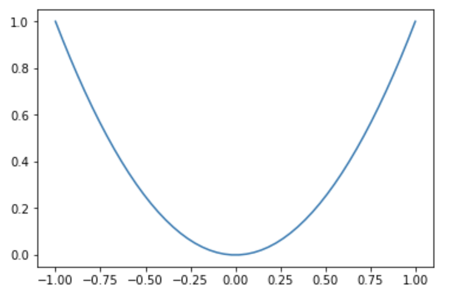
import matplotlib.pyplot as plt
import numpy as np
x = np.linspace(-3,3,50)
y1 = 2*x + 1
y2 = x**2

plt.figure()
plt.plot(x,y1)

# plt.figure()
plt.figure(num = 3, figsize = [8,5])
plt.plot(x,y2)
plt.plot(x,y1,color = 'red', linewidth = 1.0, linestyle = '--')
plt.show()
import matplotlib.pyplot as plt
import numpy as np
x = np.linspace(-3,3,50)
y1 = 2*x + 1
y2 = x**2

plt.figure(num = 3, figsize = [8,5])

plt.xlim((-1,2))
plt.ylim((-2,3))
plt.xlabel('I am X')
plt.ylabel('I am Y')
new_ticks = np.linspace(-1,2,5)
print(new_ticks)
plt.xticks(new_ticks)
plt.yticks([-2,-1.8,-1,1.22,3],[r'$really\ bad$',r'$bad\ \alpha$','normal','god','really good'])

#gca = 'get current axis'
ax = plt.gca()
ax.spines['right'].set_color('none')
ax.spines['top'].set_color('none')
ax.xaxis.set_ticks_position('bottom')
ax.yaxis.set_ticks_position('left')
ax.spines['bottom'].set_position(('data',0))# outward, axes
ax.spines['left'].set_position(('data',0))


l1,= plt.plot(x,y2, label = 'up')
l2,=plt.plot(x,y1,color = 'red', linewidth = 1.0, linestyle = '--',label = 'down')
# plt.legend()
plt.legend(handles=[l1,l2,],labels=['aaa','bbb'],loc='best')
plt.show()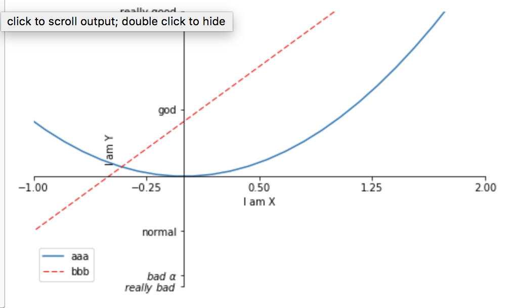
import matplotlib.pyplot as plt
import numpy as np

x = np.linspace(-3,3,50)
y = 2*x + 1

plt.figure(num=1,figsize=(8,5),)
plt.plot(x,y,)
# plt.scatter(x,y,)

ax = plt.gca()
ax.spines['right'].set_color('none')
ax.spines['top'].set_color('none')
ax.xaxis.set_ticks_position('bottom')
ax.spines['bottom'].set_position(('data',0))
ax.yaxis.set_ticks_position('left')
ax.spines['left'].set_position(('data',0))

x0 = 1
y0 = 2*x0 + 1
plt.scatter(x0,y0,s=50,color='b')
plt.plot([x0,x0],[y0,0],'k--',lw=2.5)

#method 1
plt.annotate(r'$2x+1 = %s$'% y0,xy=(x0,y0),xycoords='data',xytext=(+30,-30),textcoords = 'offset points',fontsize=16,arrowprops=dict(arrowstyle='->',connectionstyle='arc3,rad=.2'))
#method 2
plt.text(-3.7,3,r'$This\ is\ the\ some\ text.\ \mu\ \sigma_i\ \alpha_t$',fontdict={'size':16,'color':'r'})
plt.show()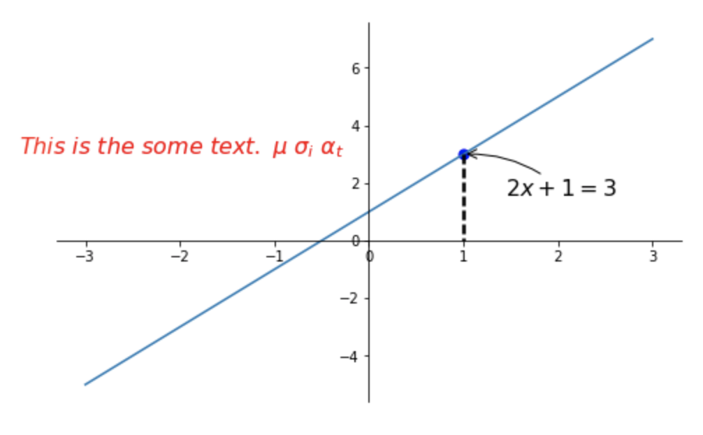
# 散点数据
import matplotlib.pyplot as plt
import numpy as np
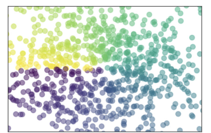
n = 1024
X = np.random.normal(0,1,n)
Y = np.random.normal(0,1,n)
T = np.arctan2(Y,X)# for color value
plt.scatter(X,Y,s=75,c=T,alpha =0.5)
# plt.scatter(np.arange(5),np.arange(5))
plt.xlim((-1.5,1.5))
plt.ylim((-1.5,1.5))
plt.xticks(())
plt.yticks(())
plt.show()
import matplotlib.pyplot as plt
import numpy as np

n = 12
X = np.arange(n)
Y1=(1-X/float(n)) * np.random.uniform(0.5,1.0,n)
Y2=(1-X/float(n)) * np.random.uniform(0.5,1.0,n)

plt.bar(X,+Y1,facecolor='#9999ff',edgecolor='white')
plt.bar(X,-Y2,facecolor='#ff9999',edgecolor='white')

for x,y in zip(X,Y1):
    #ha: horizontal alignment
    plt.text(x ,y+ 0.05,'%.2f'%y,ha='center',va ='bottom')

for x,y in zip(X,Y2):
    #ha: horizontal alignment
    plt.text(x,-y- 0.05,'-%.2f'%y,ha='center',va ='top')

plt.xlim(-.5,n)
plt.xticks(())
plt.ylim(-1.25,1.25)
plt.yticks(())

plt.show()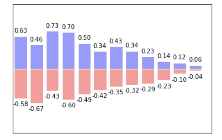
import matplotlib.pyplot as plt
import numpy as np

def f(x,y):
    #the height function
    return (1-x/2 + x**5 + y**3)*np.exp(-x**2-y**2)

n = 256
x = np.linspace(-3,3,n)
y = np.linspace(-3,3,n)
X,Y = np.meshgrid(x,y)

#use plt.contourf to filling contours
#X,Y and value for (X,Y) point
plt.contourf(X,Y,f(X,Y),8,alpha = 0.75, cmap = plt.cm.hot)

#use plt.contour to add contour lines
C = plt.contour(X,Y,f(X,Y),8,colors='black',linewidth = .5)

# adding label
plt.clabel(C,inline = True,fontsize=10)

plt.xticks(())
plt.yticks(())
plt.show()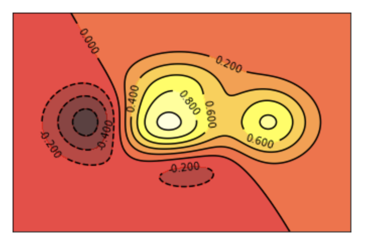
import matplotlib.pyplot as plt
import numpy as np

#image data
a = np.array([0.313660827978,0.365348418405,0.423733120134,
             0.365348418405,0.439599930621,0.525083754405,
             0.423733120134,0.525083754405,0.651536351379]).reshape(3,3)

plt.imshow(a,interpolation ='nearest',cmap ='bone',origin='lower')
# plt.colorbar()
plt.colorbar(shrink=0.9)

plt.xticks(())
plt.yticks(())
plt.show()
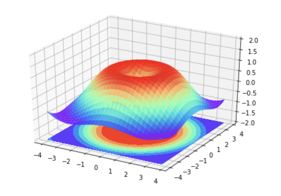
import numpy as np
import matplotlib.pyplot as plt
from mpl_toolkits.mplot3d import Axes3D

fig = plt.figure()
ax = Axes3D(fig)
X = np.arange(-4,4,0.25)
Y = np.arange(-4,4,0.25)
X,Y = np.meshgrid(X,Y)
R = np.sqrt(X **2 + Y **2)

Z = np.sin(R)

ax.plot_surface(X,Y,Z,rstride = 1,cstride = 1,cmap = plt.get_cmap('rainbow'))
ax.contourf(X,Y,Z,zdir='z',offset= -2, cmap='rainbow')
ax.set_zlim(-2,2)

plt.show()

import matplotlib.pyplot as plt
import matplotlib.gridspec as gridspec

#method 1:subplot2grid
# plt.figure()
# ax1 = plt.subplot2grid((3,3),(0,0),colspan =3,rowspan =1)
# ax1.plot([1,2],[1,2])
# ax1.set_xlabel('ax1_title')
# ax2 = plt.subplot2grid((3,3),(1,0),colspan =2)
# ax3 = plt.subplot2grid((3,3),(1,2),rowspan =2)
# ax4 = plt.subplot2grid((3,3),(2,0))
# ax4 = plt.subplot2grid((3,3),(2,1))

#method 2:gridspec
# plt.figure()
# gs = gridspec.GridSpec(3,3)
# ax1 = plt.subplot(gs[0,:])
# ax2 = plt.subplot(gs[1,:2])
# ax3 = plt.subplot(gs[1:,2])
# ax4 = plt.subplot(gs[-1,0])
# ax5 = plt.subplot(gs[-1,-2])

#method 3:easy to define structure
f,((ax11,ax12),(ax21,ax22))= plt.subplots(2,2,sharex = True,sharey = True)
ax11.scatter([1,2],[1,2])

plt.tight_layout()
plt.show()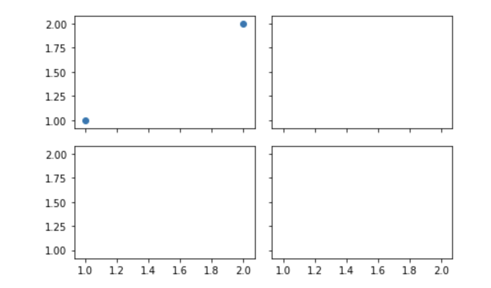
import matplotlib.pyplot as plt

fig = plt.figure()
x = [1,2,3,4,5,6,7]
y = [1,3,4,2,5,8,6]

left, bottom, width, height = 0.1,0.1,0.8,0.8
ax1 = fig.add_axes([left, bottom, width, height])
ax1.plot(x,y,'r')
ax1.set_xlabel('x')
ax1.set_ylabel('y')
ax1.set_title('title')


left, bottom, width, height = 0.2,0.6,0.25,0.25
ax2 = fig.add_axes([left, bottom, width, height])
ax2.plot(x,y,'b')
ax2.set_xlabel('x')
ax2.set_ylabel('y')
ax2.set_title('title inside 1')


plt.axes([0.6,0.2,0.25,0.25])
plt.plot(y[::-1],x,'g')
plt.xlabel('x')
plt.ylabel('y')
plt.title('title inside 2')

plt.show()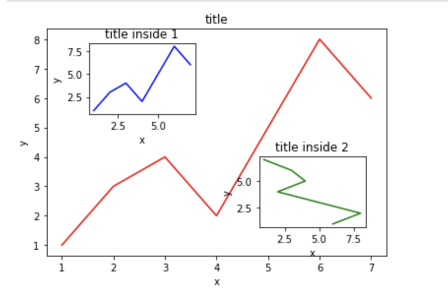
import matplotlib.pyplot as plt
import numpy as np

x = np.arange(0,10,0.1)
y1 = 0.05 * x**2
y2 = -1 * y1

fig,ax1 = plt.subplots()
ax2 = ax1.twinx()
ax1.plot(x,y1,'g-')
ax2.plot(x,y2,'b--')

ax1.set_xlabel('X data')
ax1.set_ylabel('Y1',color ='g')
ax2.set_ylabel('Y2',color='b')


plt.show()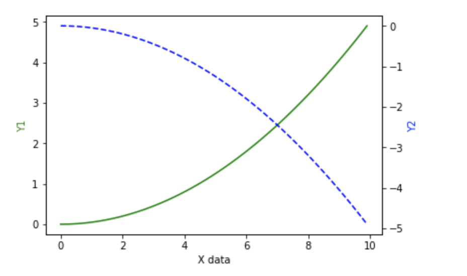
import numpy as np
from matplotlib import pyplot as plt
from matplotlib import animation

fig, ax = plt.subplots()
x = np.arange(0,2*np.pi,0.01)
line,=ax.plot(x,np.sin(x))

def animate(i):
    line.set_ydata(np.sin(x + i/10))
    return line,
def init():
    line.set_ydata(np.sin(x))
    return line,

ani = animation.FuncAnimation(fig = fig,func=animate,frames=100,init_func=init,interval=20,blit=False)
# %matplotlib nbagg
plt.show()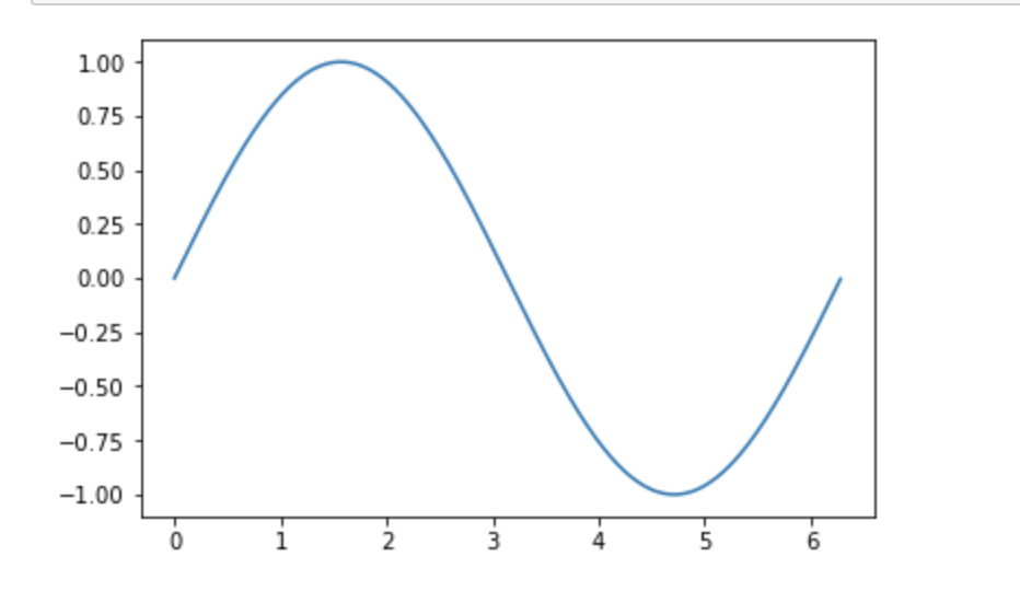
原视频地址:https://www.youtube.com/watch?v=0g-AuWBTnyg&list=PLXO45tsB95cKiBRXYqNNCw8AUo6tYen3l&index=19


 2982
2982


 被折叠的 条评论
为什么被折叠?
被折叠的 条评论
为什么被折叠?
 到【灌水乐园】发言


