信息可视化与可视分析_文字分析和可视化

信息可视化与可视分析

For this post, I want to describe a text analytics and visualization technique using a basic keyword extraction mechanism using nothing but a word counter to find the top 3 keywords from a corpus of articles that I’ve created from my blog at http://ericbrown.com.  To create this corpus, I downloaded all of my blog posts (~1400 of them) and grabbed the text of each post. Then, I tokenize the post using nltk and various stemming / lemmatization techniques, count the keywords and take the top 3 keywords.  I then aggregate all keywords from all posts to create a visualization using Gephi.

对于这篇文章，我想描述一种文本分析和可视化技术，它使用一种基本的关键字提取机制，仅使用一个单词计数器来从我在http：//博客中创建的一组文章中查找前3个关键字。 ericbrown.com。 为了创建这个语料库，我下载了所有博客文章（其中约1400个），并获取了每个文章的文本。 然后，我使用nltk和各种词干/词形化技术对帖子进行标记化，计算关键字并选择前3个关键字。 然后，我汇总所有帖子中的所有关键字，以使用Gephi创建可视化效果 。

I’ve uploaded a jupyter notebook with the full code-set for you to replicate this work. You can also get a subset of my blog articles in a csv file here.   You’ll need beautifulsoup and nltk installed. You can install them with:

我已经上传了具有完整代码集的jupyter笔记本，以供您复制此工作 。 您还可以在此处的csv文件中获取我的博客文章的子集。 您将需要安装beautifulsoup和nltk。 您可以使用以下方法安装它们：

pip install bs4 nltk

To get started, let’s load our libraries:

首先，让我们加载我们的库：

import pandas as pd
import numpy as np

from nltk.tokenize import word_tokenize, sent_tokenize
from nltk.corpus import stopwords
from nltk.stem import WordNetLemmatizer, PorterStemmer
from string import punctuation
from collections import Counter

from collections import OrderedDict
import re
import warnings
warnings.filterwarnings("ignore", category=DeprecationWarning)

from HTMLParser import HTMLParser
from bs4 import BeautifulSoup

I’m loading warnings here because there’s a warning about BeautifulSoup that we can ignore.

我在这里加载警告，因为有关于 BeautifulSoup 我们可以忽略。

Now, let’s set up some things we’ll need for this work.

现在，让我们为这项工作设置一些我们需要的东西。

First, let’s set up our stop words, stemmers and lemmatizers.

首先，让我们设置停用词，词干提取器和词义提取器。

porter = PorterStemmer()
wnl = WordNetLemmatizer() 
stop = stopwords.words('english')
stop.append("new")
stop.append("like")
stop.append("u")
stop.append("it'")
stop.append("'s")
stop.append("n't")
stop.append('mr.')
stop = set(stop)

Now, let’s set up some functions we’ll need.

现在，让我们设置一些我们需要的功能。

The tokenizer function is taken from here.  If you want to see some cool topic modeling, jump over and read How to mine newsfeed data and extract interactive insights in Python…its a really good article that gets into topic modeling and clustering…which is something I’ll hit on here as well in a future post.

标记器功能取自此处 。 如果您想看一些很酷的主题建模，请跳过并阅读如何在Python中挖掘新闻提要数据并提取交互式见解 ……这是一篇非常不错的文章，它涉及主题建模和集群化……这也是我在这里要谈到的内容。在以后的帖子中。

# From http://ahmedbesbes.com/how-to-mine-newsfeed-data-and-extract-interactive-insights-in-python.html

def tokenizer(text):

    tokens_ = [word_tokenize(sent) for sent in sent_tokenize(text)]

    tokens = []
    for token_by_sent in tokens_:
        tokens += token_by_sent

    tokens = list(filter(lambda t: t.lower() not in stop, tokens))
    tokens = list(filter(lambda t: t not in punctuation, tokens))
    tokens = list(filter(lambda t: t not in [u"'s", u"n't", u"...", u"''", u'``', u'u2014', u'u2026', u'u2013'], tokens))
     
    filtered_tokens = []
    for token in tokens:
        token = wnl.lemmatize(token)
        if re.search('[a-zA-Z]', token):
            filtered_tokens.append(token)

    filtered_tokens = list(map(lambda token: token.lower(), filtered_tokens))

    return filtered_tokens

Next, I had some html in my articles, so i wanted to strip it from my text before doing anything else with it…here’s a class to do that using bs4.  I found this code on Stackoverflow.

接下来，我在文章中添加了一些html，因此在进行其他操作之前，我想将其从文本中剥离出来……这是一个使用bs4进行此操作的类。 我在Stackoverflow上找到了这段代码。

class MLStripper(HTMLParser):
    def __init__(self):
        self.reset()
        self.fed = []
    def handle_data(self, d):
        self.fed.append(d)
    def get_data(self):
        return ''.join(self.fed)

def strip_tags(html):
    s = MLStripper()
    s.feed(html)
    return s.get_data()

OK – now to the fun stuff. To get our keywords, we need only 2 lines of code. This function does a count and returns said count of keywords for us.

好-现在到有趣的东西。 要获取关键字，我们只需要两行代码。 此函数进行计数并为我们返回关键字的所述计数。

def get_keywords(tokens, num):
    return Counter(tokens).most_common(num)

Finally,  I created a function to take a pandas dataframe filled with urls/pubdate/author/text and then create my keywords from that.  This function  iterates over a pandas dataframe (each row is an article from my blog), tokenizes the ‘text’ from  and returns a pandas dataframe with keywords, the title of the article and the publication data of the article.

最后，我创建了一个函数来获取填充了urls / pubdate / author / text的pandas数据框，然后从中创建关键字。 此函数遍历pandas数据框（每一行是我博客中的文章），标记化来自的“文本”，并返回带有关键字，文章标题和文章的发布数据的pandas数据框。

def build_article_df(urls):
    articles = []
    for index, row in urls.iterrows():
        try:
            data=row['text'].strip().replace("'", "")
            data = strip_tags(data)
            soup = BeautifulSoup(data)
            data = soup.get_text()
            data = data.encode('ascii', 'ignore').decode('ascii')
            document = tokenizer(data)
            top_5 = get_keywords(document, 5)
          
            unzipped = zip(*top_5)
            kw= list(unzipped[0])
            kw=",".join(str(x) for x in kw)
            articles.append((kw, row['title'], row['pubdate']))
        except Exception as e:
            print e
            #print data
            #break
            pass
        #break
    article_df = pd.DataFrame(articles, columns=['keywords', 'title', 'pubdate'])
    return article_df

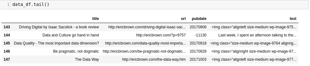
Time to load the data and start analyzing. This bit of code loads in my blog articles (found here) and then grabs only the interesting columns from the data, renames them and prepares them for tokenization. Most of this can be done in one line when reading in the csv file, but I already had this written for another project and just it as is.

是时候加载数据并开始分析了。 这些代码加载到我的博客文章中（在此处找到），然后仅从数据中获取有趣的列，对其进行重命名并为进行标记化做准备。 读取csv文件时，大多数操作都可以在一行中完成，但是我已经将它写在了另一个项目中，并保持原样。

df = pd.read_csv('../examples/tocsv.csv')
data = []
for index, row in df.iterrows():
    data.append((row['Title'], row['Permalink'], row['Date'], row['Content']))
data_df = pd.DataFrame(data, columns=['title' ,'url', 'pubdate', 'text' ])

Taking the tail() of the dataframe gets us:

以 tail() 的数据帧使我们：

Now, we can tokenize and do our word-count by calling our build_article_df function.

现在，我们可以通过调用 build_article_df 功能。

article_df = build_article_df(data_df)

This gives us a new dataframe with the top 3 keywords for each article (along with the pubdate and title of the article).

这为我们提供了一个新的数据框，其中包含每篇文章的前3个关键字（以及文章的发布日期和标题）。

 

 

 

 

 

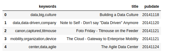
This is quite cool by itself. We’ve generated keywords for each article automatically using a simple counter. Not terribly sophisticated but it works and works well. There are many other ways to do this, but for now we’ll stick with this one. Beyond just having the keywords, it might be interesting to see how these keywords are ‘connected’ with each other and with other keywords. For example, how many times does ‘data’ shows up in other articles?

它本身就很酷。 我们已经使用一个简单的计数器自动为每篇文章生成了关键字。 虽然不是很复杂，但是它可以正常工作。 还有许多其他方法可以执行此操作，但现在我们将继续使用此方法。 除了拥有关键字之外，看看这些关键字如何彼此“相互连接”以及与其他关键字“连接”起来可能很有趣。 例如，“数据”在其他文章中出现了多少次？

There are multiple ways to answer this question, but one way is by visualizing the keywords in a topology / network map to see the connections between keywords. we need to do a ‘count’ of our keywords and then build a co-occurrence matrix. This matrix is what we can then import into Gephi to visualize. We could draw the network map using networkx, but it tends to be tough to get something useful from that without a lot of work…using Gephi is much more user friendly.

有多种方法可以回答这个问题，但是一种方法是通过可视化拓扑/网络图中的关键字来查看关键字之间的连接。 我们需要对关键字进行“计数”，然后建立一个共现矩阵。 然后可以将这个矩阵导入Gephi进行可视化。 我们可以使用networkx来绘制网络图，但是如果不付出大量工作就很难从中获得有用的信息……使用Gephi更加用户友好。

We have our keywords and need a co-occurance matrix. To get there, we need to take a few steps to get our keywords broken out individually.

我们有关键字，并且需要一个共现矩阵。 要到达那里，我们需要采取一些步骤来分别分解关键字。

keywords_array=[]
for index, row in article_df.iterrows():
    keywords=row['keywords'].split(',')
    for kw in keywords:
        keywords_array.append((kw.strip(' '), row['keywords']))
kw_df = pd.DataFrame(keywords_array).rename(columns={0:'keyword', 1:'keywords'})

We now have a keyword dataframe kw_df that holds two columns: keyword and keywords with keyword

现在，我们有了一个关键字数据框 kw_df 包含两列：关键字和带有的关键字 keyword

 

 

 

 

 

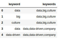
This doesn’t really make a lot of sense yet, but we need both columns to build a co-occurance matrix. We do by iterative over each document keyword list (the keywords column) and seeing if the keyword is included. If so, we added to our occurance matrix and then build our co-occurance matrix.

这实际上并没有多大意义，但是我们需要两列来建立共存矩阵。 我们通过迭代每个文档关键字列表（ keywords 列），然后查看 keyword 已经包括了。 如果是这样，我们将其添加到发生矩阵中，然后构建我们的共现矩阵。

document = kw_df.keywords.tolist()
names = kw_df.keyword.tolist()

document_array = []
for item in document:
    items = item.split(',')
    document_array.append((items))

occurrences = OrderedDict((name, OrderedDict((name, 0) for name in names)) for name in names)

# Find the co-occurrences:
for l in document_array:
    for i in range(len(l)):
        for item in l[:i] + l[i + 1:]:
            occurrences[l[i]][item] += 1

co_occur = pd.DataFrame.from_dict(occurrences )

Now, we have a co-occurance matrix in the co_occur dataframe, which can be imported into Gephi to view a map of nodes and edges. Save the co_occur dataframe as a CSV file for use in Gephi (you can download a copy of the matrix here).

现在，我们在 co_occur 数据框，可以将其导入Gephi以查看节点和边缘的地图。 保存 co_occur 数据框作为供Gephi使用的CSV文件（您可以在此处下载矩阵的副本）。

co_occur.to_csv('out/ericbrown_co-occurancy_matrix.csv')

到Gephi (Over to Gephi)

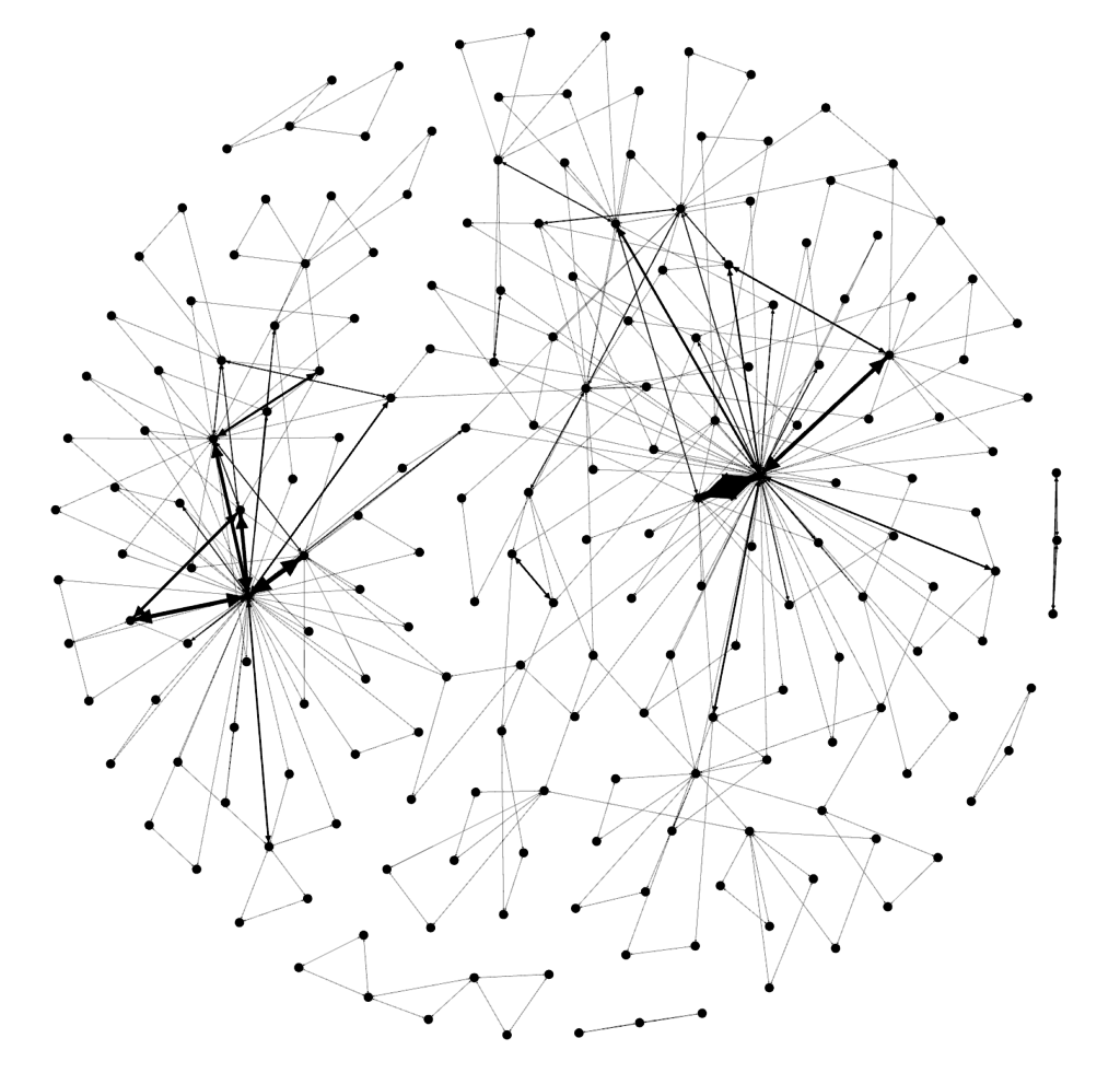
Now, its time to play around in Gephi. I’m a novice in the tool so can’t really give you much in the way of a tutorial, but I can tell you the steps you need to take to build a network map. First, import your co-occuance matrix csv file using File -> Import Spreadsheet and just leave everything at the default.  Then, in the ‘overview’ tab, you should see a bunch of nodes and connections like the image below.

现在，该在Gephi玩游戏了。 我是该工具的新手，因此实际上并不能给您太多指导，但是我可以告诉您构建网络映射所需的步骤。 首先，使用文件->导入电子表格导入同频矩阵csv文件，并将所有内容保留为默认值。 然后，在“概述”选项卡中，您应该看到一堆节点和连接，如下图所示。

Network map of a subset of ericbrown.com articles

ericbrown.com文章子集的网络图

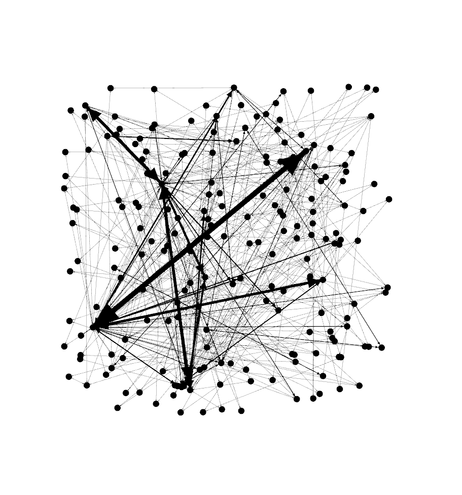
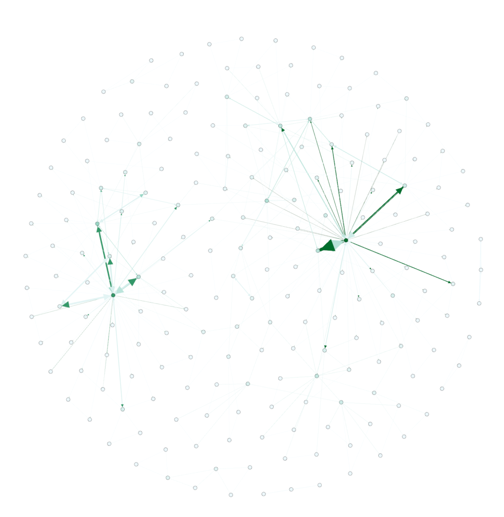
Next, move down to the ‘layout’ section and select the Fruchterman Reingold layout and push ‘run’ to get the map to redraw. At some point, you’ll need to press ‘stop’ after the nodes settle down on the screen. You should see something like the below.

接下来，移至“版式”部分，选择Fruchterman Reingold版式，然后按“运行”以重绘地图。 在某些时候，您需要在节点在屏幕上停下来后按“停止”。 您应该看到类似下面的内容。

Network map of a subset of ericbrown.com articles

ericbrown.com文章子集的网络图

 

Cool, huh? Now…let’s get some color into this graph.  In the ‘appearance’ section, select ‘nodes’ and then ‘ranking’. Select “Degree’ and hit ‘apply’.  You should see the network graph change and now have some color associated with it.  You can play around with the colors if you want but the default color scheme should look something like the following:

酷吧？ 现在...让我们在此图中添加一些颜色。 在“外观”部分中，选择“节点”，然后选择“排名”。 选择“同意”并点击“应用”。 您应该看到网络图发生了变化，并且现在有了一些关联的颜色。 如果需要，可以尝试使用颜色，但是默认的配色方案应类似于以下内容：

Still not quite interesting though. Where’s the text/keywords?  Well…you need to swtich over to the ‘overview’ tab to see that. You should see something like the following (after selecting ‘Default Curved’ in the drop-down.

仍然不是很有趣。 文字/关键字在哪里？ 好吧……您需要转到“概述”标签才能看到它。 您应该看到类似以下的内容（在下拉菜单中选择“默认弯曲”后）。

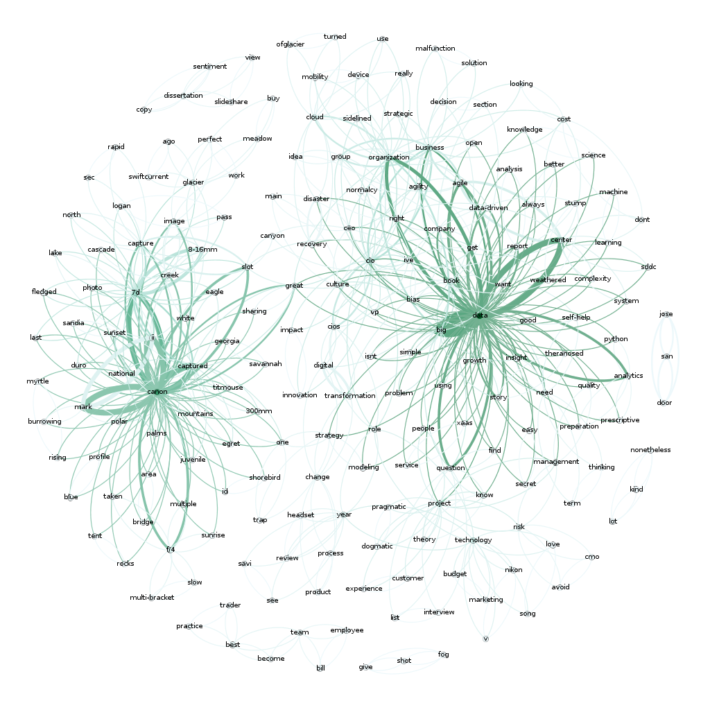
Now that’s pretty cool. You can see two very distinct areas of interest here. “Data’ and “Canon”…which makes sense since I write a lot about data and share a lot of my photography (taken with a Canon camera).

现在，这很酷。 您可以在此处看到两个非常不同的兴趣领域。 “数据”和“佳能”……之所以有意义，是因为我写了很多数据，并分享了很多我的摄影作品（用佳能相机拍摄）。

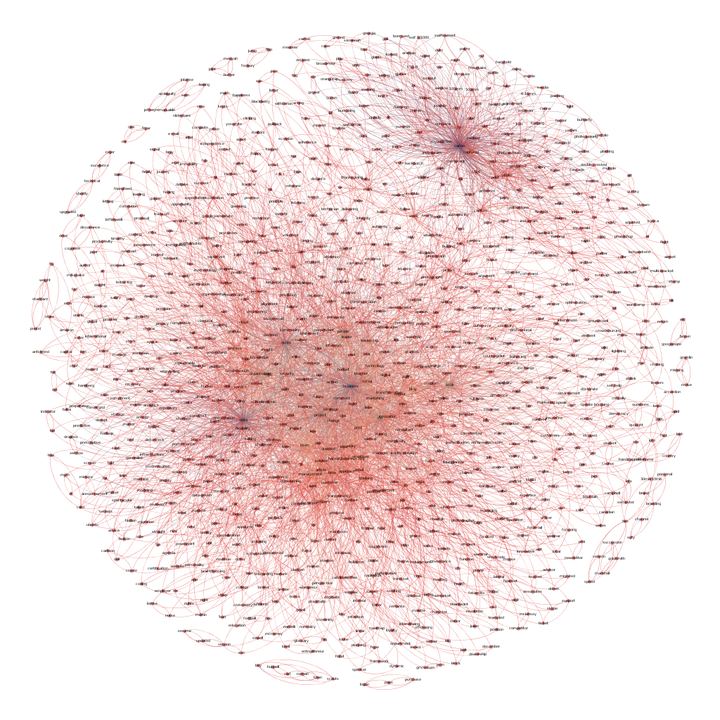
Here’s a full map of all 1400 of my articles if you are interested.  Again, there are two main clusters around photography and data but there’s also another large cluster around ‘business’, ‘people’ and ‘cio’, which fits with what most of my writing has been about over the years.

如果您有兴趣，这是我所有1400篇文章的完整地图。 同样，围绕摄影和数据有两个主要的集群，但是围绕“商业”，“人”和“ cio”的还有另一个大集群，这与我多年来的大部分写作相吻合。

There are a number of other ways to visualize text analytics.  I’m planning a few additional posts to talk about some of the more interesting approaches that I’ve used and run across recently. Stay tuned.

还有许多其他方式可以可视化文本分析。 我正在计划其他几篇文章，以讨论我最近使用和遇到的一些更有趣的方法。 敬请关注。

---

---

If you want to learn more about Text analytics, check out these books:

如果您想了解有关文本分析的更多信息，请查看以下书籍：

Text Analytics with Python: A Practical Real-World Approach to Gaining Actionable Insights from your Data 

使用Python进行文本分析：一种实用的实际方法，可从您的数据中获得可行的见解

Natural Language Processing with Python: Analyzing Text with the Natural Language Toolkit

使用Python进行自然语言处理：使用自然语言工具包分析文本

Text Mining with R

用R进行文本挖掘

---

---

 

Eric Brown 埃里克·布朗

Eric D. Brown , D.Sc. has a doctorate in Information Systems with a specialization in Data Sciences, Decision Support and Knowledge Management. He writes about utilizing python for data analytics at pythondata.com and the crossroads of technology and strategy at ericbrown.com

埃里克·布朗（Eric D.Brown） 拥有信息系统博士学位，专门研究数据科学，决策支持和知识管理。 他写了关于利用数据分析Python在 pythondata.com技术和战略的十字路口在 ericbrown.com

http://pythondata.wpengine.com/ http://pythondata.wpengine.com/

翻译自: https://www.pybloggers.com/2017/10/text-analytics-and-visualization/

信息可视化与可视分析