渲染SVG地球

您将要创造的

在本教程中，我将向您展示如何拍摄SVG地图并将其作为矢量投影到地球上。 为了执行将地图投影到球体上所需的数学转换，我们必须使用Python脚本来读取地图数据并将其转换为地球图像。 本教程假定您正在运行最新可用的Python 3.4。

Inkscape具有某种Python API，可用于执行各种操作。 但是，由于我们仅对变换形状感兴趣，因此编写一个独立的程序即可更容易，该程序可以自行读取和打印SVG文件。

1.设置地图格式

我们想要的地图类型称为等矩形图。 在等角线地图中，地点的经度和纬度与其在地图上的x和y位置相对应。 可以在Wikimedia Commons （这是带有美国各州的版本 ）上找到一个等矩形的世界地图。

SVG坐标可以通过多种方式定义。 例如，它们可以相对于先前定义的点，也可以相对于原点绝对定义。 为了使生活更轻松，我们希望将地图中的坐标转换为绝对形式。 Inkscape可以做到这一点。 转到Inkscape首选项（在“ 编辑”菜单下），然后在“ 输入/输出” >“ SVG输出”下 ，将“ 路径字符串格式”设置为“ 绝对” 。

Inkscape不会自动转换坐标。 您必须在路径上执行某种转换才能使这种情况发生。 最简单的方法是选择所有内容，然后按一下向上和向下箭头中的每一个，将其上下移动。 然后重新保存文件。

2.启动您的Python脚本

创建一个新的Python文件。 导入以下模块：

import sys
import re
import math
import time
import datetime
import numpy as np

import xml.etree.ElementTree as ET

您将需要安装NumPy ，该库可让您执行某些矢量运算，例如点积和叉积。

3.透视投影的数学

将三维空间中的点投影到2D图像中涉及找到从相机到该点的向量，然后将该向量分成三个垂直向量。

垂直于相机矢量（相机面对的方向）的两个局部矢量成为正交投影图像的x和y坐标。 平行于相机矢量的局部矢量变为点的z距离。 要将正交图像转换为透视图像，请分别将x和y坐标除以z距离。

在这一点上，定义某些相机参数是有意义的。 首先，我们需要知道相机在3D空间中的位置。 将其x ， y和z坐标存储在字典中。

camera = {'x': -15, 'y': 15, 'z': 30}

地球将位于原点，因此将照相机朝向其方位是有意义的。 这意味着相机方向向量将与相机位置相反。

cameraForward = {'x': -1*camera['x'], 'y': -1*camera['y'], 'z': -1*camera['z']}

仅仅确定相机朝向哪个方向还不够，还需要确定相机的旋转方向。 通过定义一个垂直于cameraForward向量的向量来做到这cameraForward 。

cameraPerpendicular = {'x': cameraForward['y'], 'y': -1*cameraForward['x'], 'z': 0}

1.定义有用的向量函数

在程序中定义某些矢量函数将非常有帮助。 定义矢量幅度函数：

#magnitude of a 3D vector
def sumOfSquares(vector):
    return vector['x']**2 + vector['y']**2 + vector['z']**2
def magnitude(vector):
	return math.sqrt(sumOfSquares(vector))

我们需要能够将一个向量投影到另一个向量上。 由于此操作涉及点积，因此使用NumPy库要容易得多。 但是，NumPy采用列表形式的向量，没有显式的“ x”，“ y”，“ z”标识符，因此我们需要一个函数将向量转换为NumPy向量。

#converts dictionary vector to list vector
def vectorToList (vector):
    return [vector['x'], vector['y'], vector['z']]

#projects u onto v
def vectorProject(u, v):
    return np.dot(vectorToList (v), vectorToList (u))/magnitude(v)

很高兴有一个函数可以在给定矢量的方向上为我们提供单位矢量：

#get unit vector
def unitVector(vector):
    magVector = magnitude(vector)
	return {'x': vector['x']/magVector, 'y': vector['y']/magVector, 'z': vector['z']/magVector }

最后，我们需要能够得到两个点并在它们之间找到一个向量：

#Calculates vector from two points, dictionary form
def findVector (origin, point):    
	return { 'x': point['x'] - origin['x'], 'y': point['y'] - origin['y'], 'z': point['z'] - origin['z'] }

2.定义相机轴

现在，我们只需完成定义相机轴。 我们已经有了两个这样的轴cameraForward和cameraPerpendicular ，分别对应于相机图像的z距离和x坐标。

现在我们只需要第三个轴，该轴由代表摄像机图像y坐标的矢量定义。 我们可以使用NumPy- np.cross(vectorToList(cameraForward), vectorToList(cameraPerpendicular))取这两个向量的叉积来找到第三个轴。

结果中的第一个元素对应于x分量； 第二个是y分量，第三个是z分量，因此产生的矢量由下式给出：

#Calculates horizon plane vector (points upward)
cameraHorizon = {'x': np.cross(vectorToList(cameraForward) , vectorToList(cameraPerpendicular))[0], 'y': np.cross(vectorToList(cameraForward) , vectorToList(cameraPerpendicular))[1], 'z': np.cross(vectorToList(cameraForward) , vectorToList(cameraPerpendicular))[2] }

3.投影到正交

要找到正交的x ， y和z距离，我们首先找到链接相机和所关注点的向量，然后将其投影到先前定义的三个相机轴的每一个上：

def physicalProjection (point):
    pointVector = findVector(camera, point)
		#pointVector is a vector starting from the camera and ending at a point in question
	return {'x': vectorProject(pointVector, cameraPerpendicular), 'y': vectorProject(pointVector, cameraHorizon), 'z': vectorProject(pointVector, cameraForward)}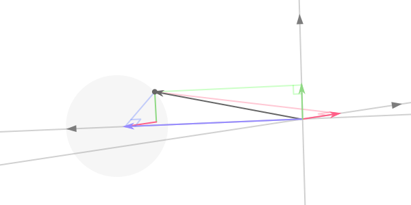

一个点（深灰色）被投影到三个相机轴（灰色）上。 x是红色， y是绿色， z是蓝色。

4.展望项目

透视投影简单地取正交投影的x和y ，然后将每个坐标除以z距离。 这样一来，距离较远的东西看上去比距离照相机更近的东西要小。

因为除以z会产生非常小的坐标，所以我们将每个坐标乘以对应于相机焦距的值。

focalLength = 1000

# draws points onto camera sensor using xDistance, yDistance, and zDistance
def perspectiveProjection (pCoords):
    scaleFactor = focalLength/pCoords['z']
	return {'x': pCoords['x']*scaleFactor, 'y': pCoords['y']*scaleFactor}

5.将球坐标转换为直角坐标

地球是一个球体。 因此，我们的坐标（经度和纬度）是球面坐标。 因此，我们需要编写一个将球坐标转换为直角坐标的函数（以及定义地球半径并提供π常数）：

radius = 10
pi = 3.14159

#converts spherical coordinates to rectangular coordinates
def sphereToRect (r, a, b):
	return {'x': r*math.sin(b*pi/180)*math.cos(a*pi/180), 'y': r*math.sin(b*pi/180)*math.sin(a*pi/180), 'z': r*math.cos(b*pi/180) }

通过存储多次使用的一些计算，我们可以提高性能：

#converts spherical coordinates to rectangular coordinates
def sphereToRect (r, a, b):
    aRad = math.radians(a)
	bRad = math.radians(b)
	r_sin_b = r*math.sin(bRad)
	return {'x': r_sin_b*math.cos(aRad), 'y': r_sin_b*math.sin(aRad), 'z': r*math.cos(bRad) }

我们可以编写一些复合函数，将前面的所有步骤组合为一个函数-直接从球形或矩形坐标到透视图图像：

#functions for plotting points
def rectPlot (coordinate):
    return perspectiveProjection(physicalProjection(coordinate))
def spherePlot (coordinate, sRadius):
	return rectPlot(sphereToRect(sRadius, coordinate['long'], coordinate['lat']))

4.渲染到SVG

我们的脚本必须能够写入SVG文件。 因此，应从以下内容开始：

f = open('globe.svg', 'w')
f.write('<?xml version=\"1.0\" encoding=\"UTF-8\"?>\n<svg viewBox="0 0 800 800" version="1.1"\nxmlns="http://www.w3.org/2000/svg" xmlns:xlink=\"http://www.w3.org/1999/xlink\">\n')

并以：

f.write('</svg>')

产生一个空但有效的SVG文件。 在该文件中，脚本必须能够创建SVG对象，因此我们将定义两个函数，以使其能够绘制SVG点和多边形：

#Draws SVG circle object
def svgCircle (coordinate, circleRadius, color):
    f.write('<circle cx=\"' + str(coordinate['x'] + 400) + '\" cy=\"' + str(coordinate['y'] + 400) + '\" r=\"' + str(circleRadius) + '\" style=\"fill:' + color + ';\"/>\n')
#Draws SVG polygon node
def polyNode (coordinate):
	f.write(str(coordinate['x'] + 400) + ',' + str(coordinate['y'] + 400) + ' ')

我们可以通过渲染点的球形网格来测试这一点：

#DRAW GRID
for x in range(72):
    for y in range(36):
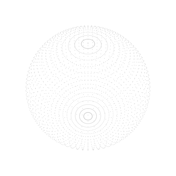
		svgCircle (spherePlot( { 'long': 5*x, 'lat': 5*y }, radius ), 1, '#ccc')

保存并运行此脚本后，应产生如下内容：

5.转换SVG地图数据

要读取SVG文件，脚本必须能够读取XML文件，因为SVG是XML的一种。 这就是为什么我们导入xml.etree.ElementTree的原因。 该模块允许您将XML / SVG作为嵌套列表加载到脚本中：

tree = ET.parse('BlankMap Equirectangular states.svg')
root = tree.getroot()

您可以通过列表索引导航到SVG中的对象（通常，您必须查看地图文件的源代码以了解其结构）。 在我们的例子中，每个国家/地区位于root[4][0][ x ][ n ] ，其中x是国家/地区的编号（从1开始），n代表概述国家/地区的各种子路径。 国家的实际轮廓存储在d属性中，可通过root[4][0][ x ][ n ].attrib['d'] 。

1.构造循环

我们不能只遍历此映射，因为它在开始时包含一个“虚拟”元素，必须跳过。 因此，我们需要计算“国家”对象的数量并减去1以摆脱虚拟对象。 然后，我们遍历其余对象。

countries = len(root[4][0]) - 1

for x in range(countries):
    root[4][0][x + 1]

一些国家对象包括多条路径，这就是为什么我们随后遍历每个国家的每条路径的原因：

countries = len(root[4][0]) - 1

for x in range(countries):
    for path in root[4][0][x + 1]:

在每个路径中， d字符串中的字符'Z M'分隔了不相交的轮廓，因此我们沿着该定界符分割d字符串，然后遍历那些定界符。

countries = len(root[4][0]) - 1

for x in range(countries):
    for path in root[4][0][x + 1]:
		for k in re.split('Z M', path.attrib['d']):

然后，我们用定界符“ Z”，“ L”或“ M”分割每个轮廓，以获取路径中每个点的坐标：

for x in range(countries):
    for path in root[4][0][x + 1]:
		for k in re.split('Z M', path.attrib['d']):
			for i in re.split('Z|M|L', k):

然后，我们从坐标中删除所有非数字字符，并沿逗号将其分成两半，以给出纬度和经度。 如果两者都存在，则将它们存储在sphereCoordinates词典中（在地图中，纬度坐标从0到180°，但是我们希望它们从–90°到90°（北和南，所以我们减去90°））。

for x in range(countries):
    for path in root[4][0][x + 1]:
		for k in re.split('Z M', path.attrib['d']):
			for i in re.split('Z|M|L', k):
				breakup = re.split(',', re.sub("[^-0123456789.,]", "", i))
				if breakup[0] and breakup[1]:
					sphereCoordinates = {}
					sphereCoordinates['long'] = float(breakup[0])
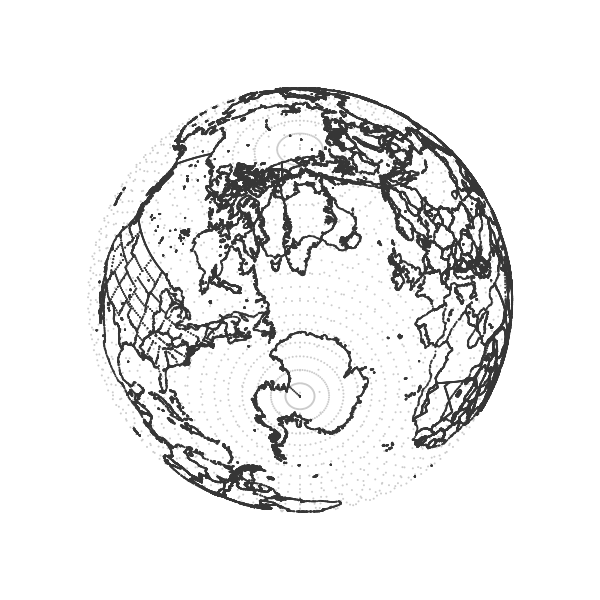
					sphereCoordinates['lat'] = float(breakup[1]) - 90

然后，如果我们通过绘制一些点来测试它（ svgCircle(spherePlot(sphereCoordinates, radius), 1, '#333') ），我们将得到如下结果：

2.解决遮挡

这不能区分地球近端的点和地球远端的点。 如果我们只想在行星的可见侧上打印点，则需要能够找出给定点在行星的哪一侧。

我们可以通过计算球体上从相机到该点的光线与球体相交的两个点来实现。 此函数实现了用于求解到这两个点dNear和dFar的距离的公式：

cameraDistanceSquare = sumOfSquares(camera)
    	#distance from globe center to camera

def distanceToPoint(spherePoint):
	point = sphereToRect(radius, spherePoint['long'], spherePoint['lat'])
	ray = findVector(camera,point)
	return vectorProject(ray, cameraForward)

def occlude(spherePoint):
    point = sphereToRect(radius, spherePoint['long'], spherePoint['lat'])
	ray = findVector(camera,point)
	d1 = magnitude(ray)
		#distance from camera to point

	dot_l = np.dot( [ray['x']/d1, ray['y']/d1, ray['z']/d1], vectorToList(camera) )
		#dot product of unit vector from camera to point and camera vector

	determinant = math.sqrt(abs( (dot_l)**2 - cameraDistanceSquare + radius**2 ))
	dNear = -(dot_l) + determinant
	dFar = -(dot_l) - determinant

如果到点的实际距离d1小于或等于这两个距离，则该点位于球体的近侧。 由于舍入错误，此操作中内置了一些摆动空间：

if d1 - 0.0000000001 <= dNear and d1 - 0.0000000001 <= dFar :
		return True
	else:
		return False

使用此功能作为条件应将渲染限制在近侧点：

if occlude(sphereCoordinates):
						svgCircle(spherePlot(sphereCoordinates, radius), 1, '#333')

6.渲染坚实的国家

当然，这些点并不是真正的封闭，填充形状-它们仅给出封闭形状的错觉。 绘制实际的填充国家需要更多的技巧。 首先，我们需要打印所有可见国家的整体。

为此，我们可以创建一个在一个国家/地区包含可见点的任何时间都会被激活的开关，同时暂时存储该国家/地区的坐标。 如果激活了开关，则使用存储的坐标绘制国家/地区。 我们还将绘制多边形而不是点。

for x in range(countries):
    for path in root[4][0][x + 1]:
    	for k in re.split('Z M', path.attrib['d']):
	
			countryIsVisible = False
			country = []
			for i in re.split('Z|M|L', k):
	
				breakup = re.split(',', re.sub("[^-0123456789.,]", "", i))
				if breakup[0] and breakup[1]:
					sphereCoordinates = {}
					sphereCoordinates['long'] = float(breakup[0])
					sphereCoordinates['lat'] = float(breakup[1]) - 90
	
					#DRAW COUNTRY
	
					if occlude(sphereCoordinates):
						country.append([sphereCoordinates, radius])
	
						countryIsVisible = True
	
					else:
						country.append([sphereCoordinates, radius])
	
			if countryIsVisible:
				f.write('<polygon points=\"')
				for i in country:
					polyNode(spherePlot(i[0], i[1]))
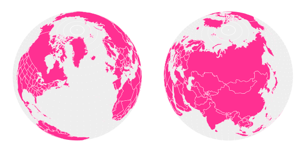
				f.write('\" style="fill:#ff3092;stroke: #fff;stroke-width:0.3\" />\n\n')

很难说，但是全球边缘的国家却自己折叠起来，这是我们不想要的（看看巴西）。

1.追踪地球的磁盘

为了使这些国家/地区在地球的边缘正确渲染，我们首先必须使用多边形跟踪地球的圆盘（您从圆点看到的圆盘是一种光学幻觉）。 圆盘由地球的可见边缘-一个圆圈勾勒出轮廓。 以下操作将计算该圆的半径和中心，以及包含该圆的平面到相机的距离以及地球的中心。

#TRACE LIMB
limbRadius = math.sqrt( radius**2 - radius**4/cameraDistanceSquare )

cx = camera['x']*radius**2/cameraDistanceSquare
cy = camera['y']*radius**2/cameraDistanceSquare
cz = camera['z']*radius**2/cameraDistanceSquare

planeDistance = magnitude(camera)*(1 - radius**2/cameraDistanceSquare)
planeDisplacement = math.sqrt(cx**2 + cy**2 + cz**2)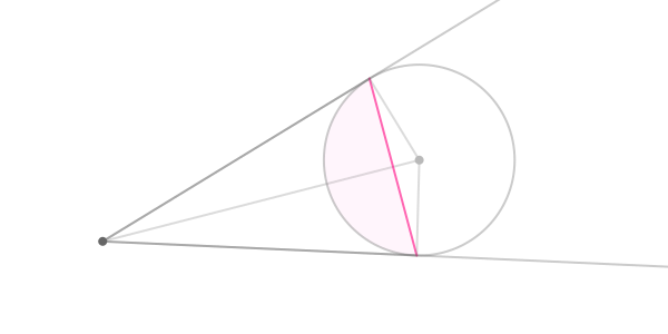

从上方观看地球和照相机（深灰点）。 粉色线代表地球的可见边缘。 相机只能看到阴影部分。

然后在该平面上绘制一个圆，我们构造了两个平行于该平面的轴：

#trade & negate x and y to get a perpendicular vector
unitVectorCamera = unitVector(camera)
aV = unitVector( {'x': -unitVectorCamera['y'], 'y': unitVectorCamera['x'], 'z': 0} )
bV = np.cross(vectorToList(aV), vectorToList( unitVectorCamera ))

然后，我们仅以2度为增量在这些轴上绘制图形，以在该平面上绘制一个具有该半径和中心的圆（有关数学信息， 请参见此说明 ）：

for t in range(180):
    theta = math.radians(2*t)
    cosT = math.cos(theta)
    sinT = math.sin(theta)
	
    limbPoint = { 'x': cx + limbRadius*(cosT*aV['x'] + sinT*bV[0]), 'y': cy + limbRadius*(cosT*aV['y'] + sinT*bV[1]), 'z': cz + limbRadius*(cosT*aV['z'] + sinT*bV[2]) }

然后，我们只用多边形绘图代码封装所有内容：

f.write('<polygon id=\"globe\" points=\"')
for t in range(180):
    theta = math.radians(2*t)
	cosT = math.cos(theta)
	sinT = math.sin(theta)
	
	limbPoint = { 'x': cx + limbRadius*(cosT*aV['x'] + sinT*bV[0]), 'y': cy + limbRadius*(cosT*aV['y'] + sinT*bV[1]), 'z': cz + limbRadius*(cosT*aV['z'] + sinT*bV[2]) }

	polyNode(rectPlot(limbPoint))

f.write('\" style="fill:#eee;stroke: none;stroke-width:0.5\" />')

我们还创建了该对象的副本，以后将其用作我们所有国家/地区的剪贴蒙版：

f.write('<clipPath id=\"clipglobe\"><use xlink:href=\"#globe\"/></clipPath>')

那应该给你这个：

2.裁剪到磁盘

使用新计算的磁盘，我们可以在国家/地区绘图代码中修改else语句（当坐标位于地球的隐藏侧时）以将这些点绘制在磁盘之外的某个位置：

else:
						tangentscale = (radius + planeDisplacement)/(pi*0.5)
						rr = 1 + abs(math.tan( (distanceToPoint(sphereCoordinates) - planeDistance)/tangentscale ))
						country.append([sphereCoordinates, radius*rr])

这使用切线曲线将隐藏点提升到地球表面上方，使它们看起来像散布在地球周围：

这在数学上并不完全是声音（如果照相机未大致对准行星的中心，它会崩溃），但是它很简单并且在大多数情况下都有效。 然后，只需将clip-path="url(#clipglobe)"到多边形绘图代码中，就可以将国家/地区整齐地裁剪到地球的边缘：

if countryIsVisible:
				f.write('<polygon clip-path="url(#clipglobe)" points=\"')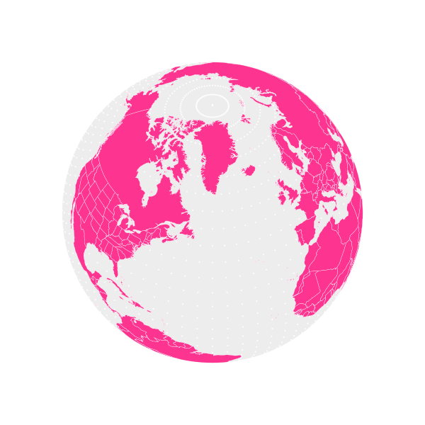

希望您喜欢本教程！ 玩转您的矢量地球仪吧！

翻译自: https://code.tutsplus.com/tutorials/render-an-svg-globe--cms-24275