


一、准备工作
- 安装Ipython Notebook[4]
- 设置远程访问服务器上Ipython[2,5],我直接用的[5]中的方法,可以直接在本地浏览器上使用服务器上的notebook。
- 在工作目录下输入命令 jupyter notebook --ip 0.0.0.0
- 会输出一个同token,在浏览器上输入服务器ip和token组成的URL,例如:http://192.168.2.175:8888/tree?token=b63ad6d9c7ee1877bd2bdeb5060ceb9e4e250644a311e948
- 学习IPython Notebook教程[7,8]
- 建立课程作业的anaconda环境[6]
- 要设置虚拟环境,请运行(在终端中)
conda create -n cs231n python=3.6 anaconda创建一个叫做的环境cs231n。 - 要激活并进入环境,请运行
source activate cs231n - 要退出,您只需关闭窗口或运行即可
source deactivate cs231n - 请注意,每次要处理作业时,都应该运行
source activate cs231n
- 要设置虚拟环境,请运行(在终端中)
- 下载数据:
cd cs231n/datasets

./get_datasets.sh
Q1:k-最近邻分类器(20分)
IPython Notebook knn.ipynb将引导您完成kNN分类器的实现。
Step1: 在Jupyter中打开knn.ipnb
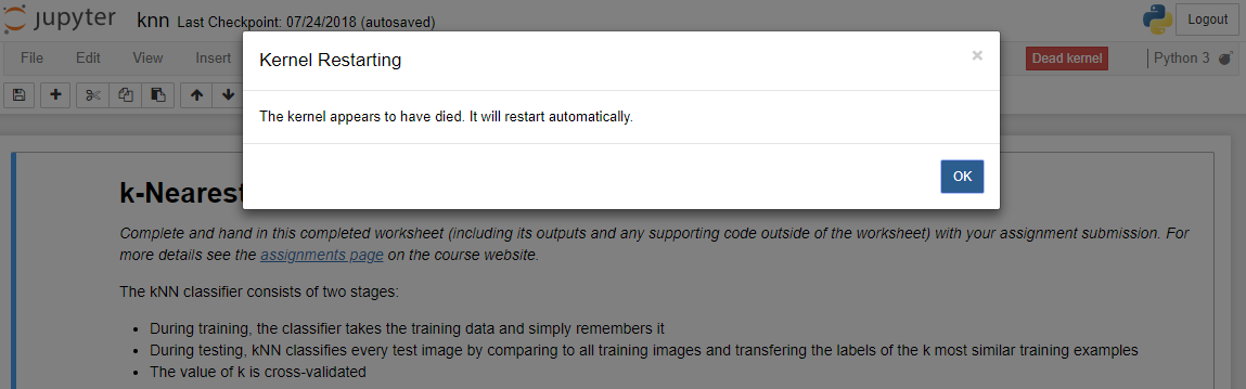
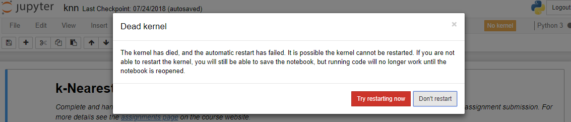
出现问题:
Kernel崩溃,如下图所示,Ipython浏览器里报错:“The kernel has died, and the automatic restart has failed. It is possible the kernel cannot be restarted. If you are not able to restart the kernel, you will still be able to save the notebook, but running code will no longer work until the notebook is reopened.”
尝试用这个方案解决这个问题:《解决Anaconda下“The kernel has died, and the automatic restart has failed.” 的问题》,即conda更新相关库:
conda upgrade notebook
conda upgrade jupyter
再次打开 knn.ipynb 时,不再报错,问题解决。
问题描述
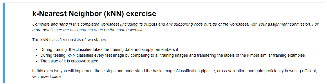
翻译:
完成工作表(包括其输出和工作表之外的任何支持代码),并与您的作业一起提交。详细信息请参阅课程网站上的作业页面。
kNN分类器包括两个阶段:
-
- 在训练期间,分类器获取训练数据并简单地记住它
- 在测试期间,kNN通过与所有训练图像进行比较并且转移k个最相似训练示例的标签来对每个测试图像进行分类
- k的值是交叉验证的
在本练习中,您将实现这些步骤并理解基本的图像分类流程、交叉验证,并提高编写高效矢量化代码的熟练程度。
Step 1: 环境参数设置
代码段1 :导入工具库
# Run some setup code for this notebook.

import random
import numpy as np
from cs231n.data_utils import load_CIFAR10
import matplotlib.pyplot as plt

from __future__ import print_function
理解:
- matplotlib是一个 Python 的 2D绘图库。通过 Matplotlib,开发者可以仅需要几行代码,便可以生成绘图,直方图,功率谱,条形图,错误图,散点图等。
- 对于image检测的Python的第一行便出现了:from __future__ import print_function原来这是为了在老版本的Python中兼顾新特性的一种方法。具体地,从python2.1开始以后, 当一个新的语言特性首次出现在发行版中时候, 如果该新特性与以前旧版本python不兼容,【9】 则该特性将会被默认禁用. 如果想启用这个新特性, 则必须使用 "from __future__import *" 语句进行导入.Python 2.7可以通过 import __future__ 来将2.7版本的print语句移除,让你可以Python3.x的print()功能函数的形式。例如:
from __future__ import print_function
print('hello', end='\t')
代码段2:设置在notebook中显示图像的默认参数
# This is a bit of magic to make matplotlib figures appear inline in the notebook
# rather than in a new window.
%matplotlib inline
plt.rcParams['figure.figsize'] = (10.0, 8.0) # set default size of plots
plt.rcParams['image.interpolation'] = 'nearest'
plt.rcParams['image.cmap'] = 'gray'
理解:
- plt.rcParams是配置参数的方法,这里inline方式实现在notebook内显示图像,接下来设置显示的默认参数【10】:
- 通过给figsize参数赋值,设置显示图像的最大范围
- 通过给interpolation赋值,设置差值方式
- 通过给cmap参数赋值'gray',设置图像在灰度空间内。
代码段3:其他设置(让notebook加载更多外部python模块)
# Some more magic so that the notebook will reload external python modules;
# see http://stackoverflow.com/questions/1907993/autoreload-of-modules-in-ipython
%load_ext autoreload
%autoreload 2
Step 2:数据的获取和处理
(1)加载原始CIFAR-10数据集
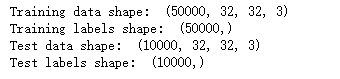
# Load the raw CIFAR-10 data.
cifar10_dir = 'cs231n/datasets/cifar-10-batches-py'

# Cleaning up variables to prevent loading data multiple times (which may cause memory issue)
try:
   del X_train, y_train
   del X_test, y_test
   print('Clear previously loaded data.')
except:
   pass

X_train, y_train, X_test, y_test = load_CIFAR10(cifar10_dir)

# As a sanity check, we print out the size of the training and test data.
print('Training data shape: ', X_train.shape)
print('Training labels shape: ', y_train.shape)
print('Test data shape: ', X_test.shape)
print('Test labels shape: ', y_test.shape)
这里使用本课程已经有的加载数据的方法加载Cifar-10数据库,首先输入数据库的路径,然后用load_CIFAR10方法自动取出训练-标记数据集和测试-标记数据集。
这里为了避免重复加载训练数据、测试数据集,用一个try-except方法处理异常。
最后做一个完成性检查,运行这个notebook单元,按下 CTRL+Enter 得到完整性检查结果:
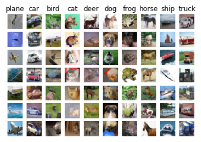
(2)可视化部分样本,显示部分训练数据样本的图像
# Visualize some examples from the dataset.
# We show a few examples of training images from each class.
classes = ['plane', 'car', 'bird', 'cat', 'deer', 'dog', 'frog', 'horse', 'ship', 'truck']
num_classes = len(classes)
samples_per_class = 7
for y, cls in enumerate(classes):
    idxs = np.flatnonzero(y_train == y)
    idxs = np.random.choice(idxs, samples_per_class, replace=False)
    for i, idx in enumerate(idxs):
        plt_idx = i * num_classes + y + 1
        plt.subplot(samples_per_class, num_classes, plt_idx)
        plt.imshow(X_train[idx].astype('uint8'))
        plt.axis('off')
        if i == 0:
            plt.title(cls)
plt.show()
该单元的运行输出:
(3)子采样:使代码运行更快
# Subsample the data for more efficient code execution in this exercise
num_training = 5000
mask = list(range(num_training))
X_train = X_train[mask]
y_train = y_train[mask]

num_test = 500
mask = list(range(num_test))
X_test = X_test[mask]
y_test = y_test[mask]
从50000张图片中取出500张作为训练样本,从10000张图片中选出500作为练习用的测试样本。
(4)将三维数据转为向量
# Reshape the image data into rows
X_train = np.reshape(X_train, (X_train.shape[0], -1))
X_test = np.reshape(X_test, (X_test.shape[0], -1))
print(X_train.shape, X_test.shape)
输出:(5000, 3072) (500, 3072)
Step 3:分类
(1)初始化KNN分类器
from cs231n.classifiers import KNearestNeighbor

# Create a kNN classifier instance.
# Remember that training a kNN classifier is a noop:
# the Classifier simply remembers the data and does no further processing
classifier = KNearestNeighbor()
classifier.train(X_train, y_train)
(2)计算距离
接下来,我们利用KNN分类器对测试数据进行分类。回忆之前我们讲过的,分类步骤包含两小步:
- 计算出所有测试数据和所有训练数据各自的距离;
- 对每一个测试样本,我们找出k个最近的样本,投票得出标签。
那么紧接着,我们先计算出这个距离矩阵。假设有 Ntr 个训练样本和 Nte 个测试样本,计算出的距离矩阵大小就是Nte*Ntr。其中,(i,j)坐标上的元素就是第i个测试样本和第j个训练样本的距离。
我们可以借助numpy提供的矩阵计算方法方便这个矩阵距离计算,但因为我对于矩阵计算的数学知识真的。。差。。。。
所以,我查阅了网上的资料来完成一层循环和无循环的计算的实现代码。
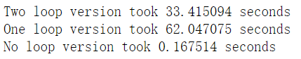
最后,在Knn.py中也计算了三个计算方法的时间。真的,巧妙地用numpy矩阵计算工具简化循环数目,可以极大地减少时间!!!
让人深深感受到numpy矩阵计算工具的神奇。要是我数学好些,或许就能玩的六很多。
以下是我对这个问题的实现:
-
两层循环计算距离:
首先,打开 cs231n/classifiers/k_nearest_neighbor.py文件, 实现compute_distances_two_loops函数。该函数在所有训练和测试样本上,利用一个双层循环计算出距离矩阵。
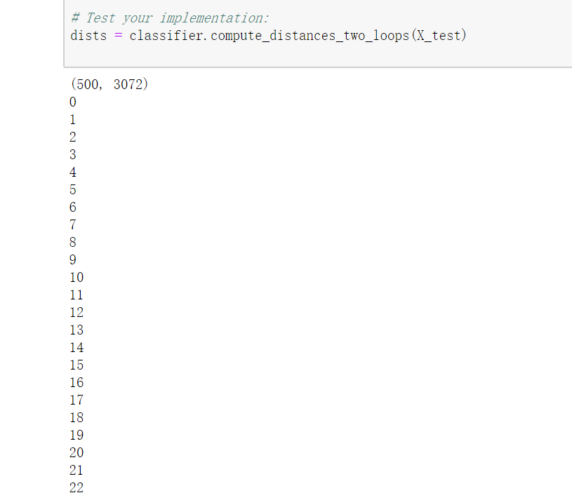
  def compute_distances_two_loops(self, X):
    """
    Compute the distance between each test point in X and each training point
    in self.X_train using a nested loop over both the training data and the
    test data.

    Inputs:
    - X: A numpy array of shape (num_test, D) containing test data.

    Returns:
    - dists: A numpy array of shape (num_test, num_train) where dists[i, j]
      is the Euclidean distance between the ith test point and the jth training
      point.
    """
    num_test = X.shape[0]
    print(X.shape)
    num_train = self.X_train.shape[0]
    dists = np.zeros((num_test, num_train))
    for i in range(num_test):
        print(i)
        for j in range(num_train):
        #####################################################################
        # TODO:                                                               #
        # Compute the l2 distance between the ith test point and the jth    #
        # training point, and store the result in dists[i, j]. You should   #
        # not use a loop over dimension.                                    #
        #####################################################################
            d = np.zeros(X.shape[1])
            for p in range(X.shape[1]):
                d[p] = np.square( X[i,p]-self.X_train[j,p])
            dists[i,j] = np.sqrt(np.sum(d))
        #####################################################################
        #                       END OF YOUR CODE                            #
        #####################################################################
    return dists
解释:
- 因为不知道什么时候程序跑得完,我加上了一个print(i),在测试Knn.py的时候,就可以知道现在正在计算第几张测试图片的距离了。事实上,我觉得这一点非常必要,因为我在运行knn.py时,单位一直显示的是“IN【*】”,说明这个单位还在被执行。就灰常滴茫然。所以我在循环里加入了这个输出,提示目前的进度。也看得出这个双层循环结构真的非常ineffficient。
- for p循环里,计算的是图片每个像素pixel相对应的训练图片中的pixel元素的距离。
- 为了实现这个东东,我还复习了一遍numpy,建议还看不懂的同学也学习下。
- 实现完以后,运行knn.py中的单元:
# Open cs231n/classifiers/k_nearest_neighbor.py and implement
# compute_distances_two_loops.

# Test your implementation:
dists = classifier.compute_distances_two_loops(X_test)
输出是这样的:
后来,我意识到对像素进行循环遍历也非常耗费时间!!!
所以参考了别人的代码,修改如下:
 def cal_dists_two_loop(self, X):
        """
        Calculate the distance with two for-loop
        Input:
        - X: A numpy array of shape (num_test, D) containing the test data
          consisting of num_test samples each of dimension D.
        Return:
        - dists: The distance between test X and train X
        """
        num_test = X.shape[0]
        num_train = self.X_train.shape[0]
        dists = np.zeros((num_test, num_train))
        for i in range(num_test):
            for j in range(num_train):
                dists[i][j] = np.sqrt(np.sum(np.square(X[i] - self.X_train[j])))

        return dists
-
一层循环计算距离:
实现compute_distances_one_loop:
   def cal_dists_one_loop(self, X):
        """
        Calculate the distance with one for-loop
        Input:
        - X: A numpy array of shape (num_test, D) containing the test data
          consisting of num_test samples each of dimension D.
        Return:
        - dists: The distance between test X and train X
        """
        num_test = X.shape[0]
        num_train = self.X_train.shape[0]
        dists = np.zeros((num_test, num_train))
        for i in range(num_test):
            dists[i] = np.sqrt(np.sum(np.square(self.X_train - X[i]), axis=1))

        return dists
-
无循环地计算距离
  def compute_distances_no_loops(self, X):
    """
    Compute the distance between each test point in X and each training point
    in self.X_train using no explicit loops.

    Input / Output: Same as compute_distances_two_loops
    """
    num_test = X.shape[0]
    num_train = self.X_train.shape[0]
    dists = np.zeros((num_test, num_train))
    #########################################################################
    # TODO:                                                                 #
    # Compute the l2 distance between all test points and all training      #
    # points without using any explicit loops, and store the result in      #
    # dists.                                                                #
    #                                                                       #
    # You should implement this function using only basic array operations; #
    # in particular you should not use functions from scipy.                #
    #                                                                       #
    # HINT: Try to formulate the l2 distance using matrix multiplication    #
    #       and two broadcast sums.                                         #
    #########################################################################
    d1 = np.multiply(np.dot(X, self.X_train.T), -2)    # shape (num_test, num_train)
    d2 = np.sum(np.square(X), axis=1, keepdims=True)    # shape (num_test, 1)
    d3 = np.sum(np.square(self.X_train), axis=1)    # shape (1, num_train)
    dists = np.sqrt(d1 + d2 + d3)
    #########################################################################
    #                         END OF YOUR CODE                              #
    #########################################################################
    return dists
-
计算每种距离计算方法的耗时:
代码是教程中已经自带的,直接运行。
# Let's compare how fast the implementations are
def time_function(f, *args):
    """
    Call a function f with args and return the time (in seconds) that it took to execute.
    """
    import time
    tic = time.time()
    f(*args)
    toc = time.time()
    return toc - tic

two_loop_time = time_function(classifier.compute_distances_two_loops, X_test)
print('Two loop version took %f seconds' % two_loop_time)

one_loop_time = time_function(classifier.compute_distances_one_loop, X_test)
print('One loop version took %f seconds' % one_loop_time)

no_loop_time = time_function(classifier.compute_distances_no_loops, X_test)
print('No loop version took %f seconds' % no_loop_time)

# you should see significantly faster performance with the fully vectorized implementation
输出:
(4)把距离可视化:
# We can visualize the distance matrix: each row is a single test example and
# its distances to training examples
plt.imshow(dists, interpolation='none')
plt.show()
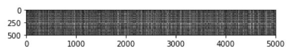
问题1:注意到距离矩阵中的结构化模式,其中某些行或列可会更亮。 (请注意,默认黑色表示距离较近,而白色表示距离较远。)
明显亮行背后的原因? 又是什么导致亮列?
你的答案:
Step 4: 预测
(1)预测标签
  def predict_labels(self, dists, k=1):
    """
    Given a matrix of distances between test points and training points,
    predict a label for each test point.

    Inputs:
    - dists: A numpy array of shape (num_test, num_train) where dists[i, j]
      gives the distance betwen the ith test point and the jth training point.

    Returns:
    - y: A numpy array of shape (num_test,) containing predicted labels for the
      test data, where y[i] is the predicted label for the test point X[i].
    """
    num_test = dists.shape[0]
    y_pred = np.zeros(num_test)

          # A list of length k storing the labels of the k nearest neighbors to
      # the ith test point.
    for i in range(num_test):
      #########################################################################
      # TODO:                                                                 #
      # Use the distance matrix to find the k nearest neighbors of the ith    #
      # testing point, and use self.y_train to find the labels of these       #
      # neighbors. Store these labels in closest_y.                           #
      # Hint: Look up the function numpy.argsort.                             #
      #########################################################################
        closest_y = []
        a = np.argsort(dists[i])[:k]
        closet_y = self.y_train[a]
        np.sort(closet_y)
      #########################################################################
      # TODO:                                                                 #
      # Now that you have found the labels of the k nearest neighbors, you    #
      # need to find the most common label in the list closest_y of labels.   #
      # Store this label in y_pred[i]. Break ties by choosing the smaller     #
      # label.                                                                #
      #########################################################################

        num_same = 0
        num_temp = 0
        for j in range(k):
            if(j == 0):
                num_same = num_temp = 1
                y_pred[i] = closet_y[0]
            else:
                if(closet_y[j] == closet_y[j-1]):
                    num_temp = num_temp + 1
                elif(closet_y[j] != closet_y[j-1]):
                    num_temp = 1
                if num_temp > num_same:
                    num_same = num_temp
                    y_pred[i] = closet_y[j]

      #########################################################################
      #                           END OF YOUR CODE                            #
      #########################################################################

    return y_pred
在knn.py中测试:
# Now implement the function predict_labels and run the code below:
# We use k = 1 (which is Nearest Neighbor).
y_test_pred = classifier.predict_labels(dists, k=1)

# Compute and print the fraction of correctly predicted examples
num_correct = np.sum(y_test_pred == y_test)
accuracy = float(num_correct) / num_test
print('Got %d / %d correct => accuracy: %f' % (num_correct, num_test, accuracy))

y_test_pred = classifier.predict_labels(dists, k=5)
num_correct = np.sum(y_test_pred == y_test)
accuracy = float(num_correct) / num_test
print('Got %d / %d correct => accuracy: %f' % (num_correct, num_test, accuracy))

Step 5: 交叉验证
Cross-validation
我们已经实现了K近邻分类器,在我们之前的代码中,我们默认k=5.现在我们通过交叉验证来决定k这个超参数的最优值。
We have implemented the k-Nearest Neighbor classifier but we set the value k = 5 arbitrarily. We will now determine the best value of this hyperparameter with cross-validation.
num_folds = 5
k_choices = [1, 3, 5, 8, 10, 12, 15, 20, 50, 100]

X_train_folds = []
y_train_folds = []
################################################################################
# TODO:                                                                        #
# Split up the training data into folds. After splitting, X_train_folds and    #
# y_train_folds should each be lists of length num_folds, where                #
# y_train_folds[i] is the label vector for the points in X_train_folds[i].     #
# Hint: Look up the numpy array_split function.                                #
################################################################################
# Your code
X_train_folds = np.array_split(X_train,num_folds)
y_train_folds = np.array_split(y_train,num_folds)
################################################################################
#                                 END OF YOUR CODE                             #
################################################################################

# A dictionary holding the accuracies for different values of k that we find
# when running cross-validation. After running cross-validation,
# k_to_accuracies[k] should be a list of length num_folds giving the different
# accuracy values that we found when using that value of k.
k_to_accuracies = {}


################################################################################
# TODO:                                                                        #
# Perform k-fold cross validation to find the best value of k. For each        #
# possible value of k, run the k-nearest-neighbor algorithm num_folds times,   #
# where in each case you use all but one of the folds as training data and the #
# last fold as a validation set. Store the accuracies for all fold and all     #
# values of k in the k_to_accuracies dictionary.                               #
################################################################################
for k in k_choices:
    accuracies = []
    for i in range(num_folds):
        Xtr = X_train_folds[:i] + X_train_folds[i+1:]
        ytr = y_train_folds[:i] + y_train_folds[i+1:]
        Xcv = X_train_folds[i]
        ycv = y_train_folds[i]
        classifier.train(Xtr,ytr)
        ycv_pred = classifier.predict(Xcv, k = k , num_loops = 1)
        accuracy = np.mean(ycv_pred == ycv)
        accuracies.append(accuracy)
    k_accuracy[k] = accuracies
################################################################################
#                                 END OF YOUR CODE                             #
################################################################################

# Print out the computed accuracies
for k in sorted(k_to_accuracies):
    for accuracy in k_to_accuracies[k]:
        print('k = %d, accuracy = %f' % (k, accuracy))
参考资料:
- 《 cs231n 课程作业 Assignment 1 》https://blog.csdn.net/zhangxb35/article/details/55223825
- 《远程访问(云)服务器上ipython设置》https://blog.csdn.net/u011531010/article/details/60580807
- 《Linux安装远程ipython notebook》https://blog.csdn.net/suzyu12345/article/details/51037905
- 《Jupyter Notebook介绍、安装及使用教程》https://www.jianshu.com/p/91365f343585
- 《本机直接远程连接服务器Jupyter notebook》https://blog.csdn.net/danlei94/article/details/74049975?utm_source=itdadao&utm_medium=referral
-
《课程设置说明
》http://cs231n.github.io/setup-instructions/ - 《Ipython教程(英文)》http://cs231n.github.io/ipython-tutorial/
- 《Jupyter notebook入门教程(上)》https://blog.csdn.net/red_stone1/article/details/72858962
-
《关于python 中的__future__模块(from __future__ import ***)》https://blog.csdn.net/wonengguwozai/article/details/75267858
-
Caffe学习1-图像识别与数据可视化:https://blog.csdn.net/cfyzcc/article/details/51318200
-
斯坦福CS231n项目实战(一):k最近邻(kNN)分类算法:https://blog.csdn.net/red_stone1/article/details/79238866
- 交叉验证(简书):https://www.jianshu.com/p/201a164e1b35


 1075
1075


 被折叠的 条评论
为什么被折叠?
被折叠的 条评论
为什么被折叠?
 到【灌水乐园】发言


