


机器学习——决策树
(一)决策树的构造
决策树(decision tree)是一类常见的机器学习算法,它是基于树结构来进行决策的。从根节点开始一步步走到叶子节点(决策)。所有的数据最终都会落到叶子节点,既可以做分类也可以做回归。
决策树构建整体流程:
- 在构造决策树时,我们需要解决的第一个问题就是,当前数据集上哪个特征在划分数据分类时起决定性作用。为了找到决定性的特征,划分出最好的结果,我们必须评估每个特征。
- 完成测试后,原始数据就被划分为几个数据子集。这些数据子集会分布在第一个决策点的所有分支上。
- 如果某个分支下的数据属于同一类型,则到这里以及正确地划分数据分类,无序进一步对数据集进行分割。
- 如果数据子集内的数据不属于同一类型,则需要重复划分数据子集的过程。
- 如何划分数据子集的算法和划分原始数据集的方法相同,直到所有具有相同类型的数据均在一个数据子集内。
划分数据集的原则是:将无需的数据变得更加有序。
1.1 信息增益
在划分数据集之前之后信息发生的变化称为信息增益(通俗理解就是特征X使得类Y的不确定性减少的程度),知道如何计算信息增益,我们就可以计算每个特征值划分数据集获得的信息增益,获得信息增益最高的特征就是最好的选择 。
在可以评测哪种数据划分方式就是最好的数据划分之前,必须学习如何计算信息增益。集合信息的度量方式称为香农熵(information gain) 或者简称为熵(entropy) 。熵是表示随机变量不确定的度量(通俗理解就是物体内部的混乱程度,不确定性越大,得到的熵值也就越大)。
熵定义为信息的期望值,在明晰这个概念之前,我们必须知道信息的定义。如果待分类的事物可能划分在多个分类之中,则符号
x
i
x_i
xi的信息定义为
l
(
x
i
)
=
−
l
o
g
2
p
(
x
i
)
l(x_{i})=-log_{2}p(x_{i})
l(xi)=−log2p(xi)
其中
p
(
x
i
)
p(x_i)
p(xi)是选择该分类的概率。
为了计算熵,我们需要计算所有类别所有可能值包含的信息期望值,通过下面的公式得到:
H
=
−
∑
i
=
1
n
p
(
x
i
)
l
o
g
2
p
(
x
i
)
H=-\sum_{i=1}^{n}p(x_{i})log_{2}p(x_{i})
H=−i=1∑np(xi)log2p(xi)
n是分类的数目。
当
p
(
x
i
)
=
0
p(x_{i})=0
p(xi)=0或
p
(
x
i
)
=
1
p(x_{i})=1
p(xi)=1时,
H
=
0
H=0
H=0,随机变量完全没有不确定性。
当
p
(
x
i
)
=
0.5
p(x_{i})=0.5
p(xi)=0.5时,
H
=
1
H =1
H=1,随机变量的不确定性最大
用Python计算熵
def calcShannonEnt(dataSet):
    numEntries = len(dataSet)
    labelCounts = {}
    for featVec in dataSet: #the the number of unique elements and their occurance
        currentLabel = featVec[-1]
        if currentLabel not in labelCounts.keys(): labelCounts[currentLabel] = 0
        labelCounts[currentLabel] += 1
    shannonEnt = 0.0
    for key in labelCounts:
        prob = float(labelCounts[key])/numEntries #可能值的期望
        shannonEnt -= prob * log(prob,2) #熵
    return shannonEnt
代码首先计算数据集的实例总数,然后创建一个数据字典,它的键值是最后一列的数值 。如果当前键值不存在,则扩展字典并将当前键值加入字典。每个键值都记录了当前类别出现的次数。最后,使用所有类标签的发生频率计算类别出现的概率。我们将用这个概率计算香农熵 ,统计所有类标签发生的次数。
用createDataSet()函数得到简单鱼鉴定数据集。
| 不浮出水面是否可以生存 | 是否有脚蹼 | 属于鱼类 | |
|---|---|---|---|
| 1 | 是 | 是 | 是 |
| 2 | 是 | 是 | 是 |
| 3 | 是 | 否 | 否 |
| 4 | 否 | 是 | 否 |
| 5 | 否 | 是 | 否 |
def createDataSet():
    """
    简单鱼鉴定数据集
    """
    dataSet = [[1, 1, 'yes'],
               [1, 1, 'yes'],
               [1, 0, 'no'],
               [0, 1, 'no'],
               [0, 1, 'no']]
    labels = ['no surfacing', 'flippers']
    return dataSet, labels
import trees
myDat, labels = trees.createDataSet()
print(myDat)
print(trees.calcShannonEnt(myDat))

熵越高,则混合的数据也越多,我们可以在数据集中添加更多的分类,观察熵是如何变化的。添加第三个名为maybe的分类,测试熵的变化:
myDat[0][-1]='maybe'
print(myDat)
print(trees.calcShannonEnt(myDat))

可以看到熵明显增大了,得到熵之后,我们就可以按照获取最大信息增益的方法划分数据集。
1.2 划分数据集
分类算法除了需要测量信息熵,还需要划分数据集,度量划分数据集的熵,以便判断当前是否正确地划分了数据集。将对每个特征划分数据集的结果计算一次信息熵,然后判断按照哪个特征划分数据集是最好的划分方式。
#按照给定特征划分数据集
def splitDataSet(dataSet, axis, value):
    """
    按照给定特征划分数据集
    :param dataSet:待划分的数据集
    :param axis:划分数据集的特征
    :param value:需要返回的特征的值
    """
    retDataSet = []                 # 创建一个新的列表对象
    for featVec in dataSet:
        if featVec[axis] == value:  # 将符合特征的数据抽取出来
            reducedFeatVec = featVec[:axis]
            reducedFeatVec.extend(featVec[axis+1:])
            retDataSet.append(reducedFeatVec)
    return retDataSet
在函数的开始声明一个新列表对象。因为该函数代码在同一数据集上被调用多次,为了不修改原始数据集,创建一个新的列表对象 。数据集这个列表中的各个元素也是列表,要遍历数据集中的每个元素,一旦发现符合要求的值,则将其添加到新创建的列表中。
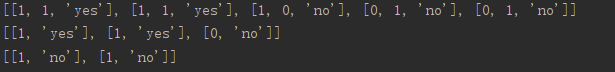
可以在简单样本数据上测试函数splitDataSet()。
myDat, labels = trees.createDataSet()
print(myDat)
print(trees.splitDataSet(myDat, 0, 1))  # 抽取,特征[0]值为1
print(trees.splitDataSet(myDat, 0, 0))  # 抽取,特征[0]值为0
接下来遍历整个数据集,循环计算熵和splitDataSet() 函数,找到最好的特征划分方式。熵计算将会告诉我们如何划分数据集是最好的数据组织方式。
def chooseBestFeatureToSplit(dataSet):
    """
    选择最好的数据集划分方式
    :param dataSet: 数据集
    :return: 返回最好特征划分的索引值
    """
    numFeatures = len(dataSet[0]) - 1      # len(dataSet[0]) 计算列数(即特征数),-1是因为最后一列是类别标签
    baseEntropy = calcShannonEnt(dataSet)  # 整个数据集的原始香农熵
    bestInfoGain = 0.0   # 初始化最好信息增益
    bestFeature = -1     # 初始化最好特征划分的索引值
    for i in range(numFeatures):        # 循环遍历数据集中的所有特征
        featList = [example[i] for example in dataSet]   # 将数据集中所有第i个特征值或者所有可能存在的值写入这个新list中
        uniqueVals = set(featList)      # 集合类型中的每个值互不相同,得到列表中唯一元素值
        newEntropy = 0.0
        for value in uniqueVals:        # 遍历当前特征中的所有唯一属性值
            subDataSet = splitDataSet(dataSet, i, value)     # 对当前特征numFeatures的每个值value划分一次数据集
            prob = len(subDataSet)/float(len(dataSet))       # 选择当前特征的当前值的概率
            newEntropy += prob * calcShannonEnt(subDataSet)  # 计算数据集的新熵值,并对所有唯一特征值得到的熵求和
        infoGain = baseEntropy - newEntropy     # 信息增益是熵的减少
        if infoGain > bestInfoGain:
            bestInfoGain = infoGain
            bestFeature = i                 # 记录最好特征划分的索引值
    return bestFeature                      # 返回最好特征划分的索引值
信息增益是熵的减少或者是数据无序度的减少,比较所有特征的信息增益,返回最好特征划分的索引值。
myDat, labels = trees.createDataSet()
print(myDat)
print(trees.chooseBestFeatureToSplit(myDat))
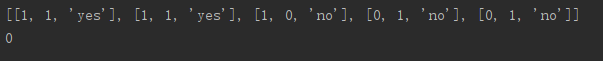
代码运行结果告诉我们,第1个特征是最好的用于划分数据集的特征。
-
如果我们按照第一个特征属性划分数据,也就是说第一个特征是1的放在一个组,第一个特征是0的放在另一个组,按照上述的方法划分数据集,第一个特征为1的海洋生物分组将有两个属于鱼类,一个属于非鱼类;另一个分组则全部属于非鱼类。
-
如果按照第二个特征分组,第一个海洋动物分组将有两个属于鱼类,两个属于非鱼类;另一个分组则只有一个非鱼类。
很明显就是第1个特征是最好的用于划分数据集的特征。
1.3 递归构建决策树
工作原理如下:得到原始数据集,然后基于最好的属性值划分数据集,由于特征值可能多于两个,因此可能存在大于两个分支的数据集划分。
第一次划分之后,数据将被向下传递到树分支的下一个节点,在这个节点上,我们可以再次划分数据。因此我们可以采用递归的原则处理数据集。
递归结束的条件是: 程序遍历完所有划分数据集的属性,或者每个分支下的所有实例都具有相同的分类。如果所有实例具有相同的分类,则得到一个叶子节点或者终止块。任何到达叶子节点的数据必然属于叶子节点的分类。
如果数据集已经处理了所有属性,但是类标签依然不是唯一的,此时我们需要决定如何定义该叶子节点,在这种情况下,我们通常会采用多数表决的方法决定该叶子节点的分类。
def majorityCnt(classList):
    """
    多数表决
    :param classList: 分类名称的列表
    :return:返回出现次数最多的分类名称
    """
    classCount = {}         # 创建键值为 classList 中唯一值的数据字典
    for vote in classList:  # 字典对象存储了 classList 中每个类标签出现的频率
        if vote not in classCount.keys():
            classCount[vote] = 0    # 没有就添加
        classCount[vote] += 1       # 次数+1
    # 利用operator操作键值降序排序字典
    sortedClassCount = sorted(classCount.items(), key=operator.itemgetter(1), reverse=True)
    return sortedClassCount[0][0]   # 返回出现次数最多的分类名称
创建树的函数代码:
def createTree(dataSet,labels):  #两个输入参数,数据集和标签列表,标签列表包含了数据集中所有特征的标签
    classList = [example[-1] for example in dataSet]  #包含了数据集的所有类别标签
    if classList.count(classList[0]) == len(classList):
        return classList[0]#stop splitting when all of the classes are equal    #所有的类标签完全相同,则直接返回该类标签
    if len(dataSet[0]) == 1: #使用完了所有特征,仍然不能将数据集划分成仅包含唯一类别的分组
        return majorityCnt(classList)
    bestFeat = chooseBestFeatureToSplit(dataSet)  #当前数据集选取的最好特征存储在变量 bestFeat 中
    bestFeatLabel = labels[bestFeat]
    myTree = {bestFeatLabel:{}}   #字典变量 myTree 存储了树的所有信息
    del(labels[bestFeat])
    featValues = [example[bestFeat] for example in dataSet]
    uniqueVals = set(featValues)
    for value in uniqueVals:
        subLabels = labels[:]       #复制了类标签,并将其存储在新列表变量 subLabels
        myTree[bestFeatLabel][value] = createTree(splitDataSet(dataSet, bestFeat, value),subLabels)
    return myTree
测试上面代码的实际输出结果:
myDat, labels = trees.createDataSet()
print(myDat)
myTree = trees.createTree(myDat, labels)
print(myTree)
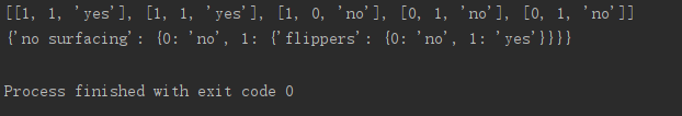
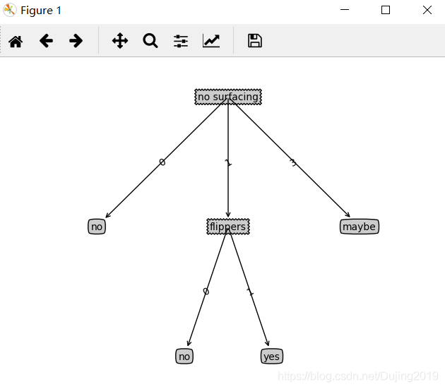
变量 myTree 包含了很多代表树结构信息的嵌套字典,从左边开始,第一个关键字 no surfacing 是第一个划分数据集的特征名称,该关键字的值也是另一个数据字典。第二个关键字是 no surfacing 特征划分的数据集,这些关键字的值是 no surfacing 节点的子节点。这些值可能是类标签(例如’flippers’),也可能是另一个数据字典。如果值是类标签,则该子节点是叶子节点;如果值是另一个数据字典,则子节点是一个判断节点,这种格式结构不断重复就构成了整棵树。这棵树包含了3个叶子节点以及2个判断节点。
(二)在 Python 中使用 Matplotlib 注解绘制树形图
2.1 Matplotlib 注解
字典的表示形式非常不易于理解,而且直接绘制图形也比较困难。现在使用Matplotlib库创建树形图。决策树的主要优点就是直观易于理解,如果不能将其直观地显示出来,就无法发挥其优势。
#使用文本注解绘制树节点
import matplotlib.pyplot as plt
decisionNode = dict(boxstyle="sawtooth", fc="0.8")
leafNode = dict(boxstyle="round4", fc="0.8")
arrow_args = dict(arrowstyle="<-")
def plotNode(nodeTxt, centerPt, parentPt, nodeType):
createPlot.ax1.annotate(nodeTxt, xy=parentPt, xycoords='axes fraction',
xytext=centerPt, textcoords='axes fraction',
va="center", ha="center", bbox=nodeType, arrowprops=arrow_args)
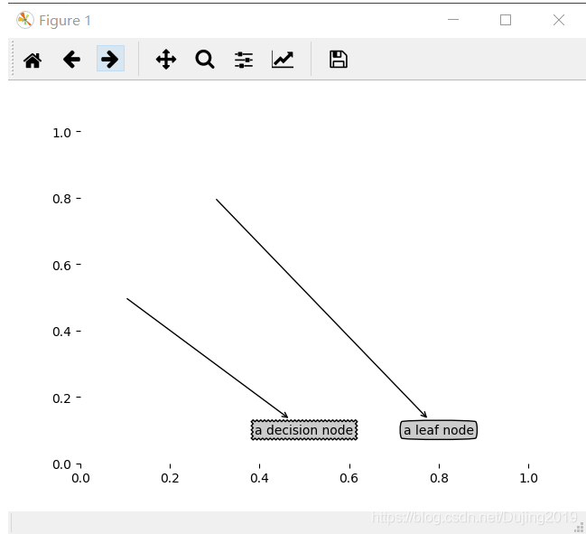
def createPlot(): #创建了一个新图形并清空绘图区,然后在绘图区上绘制两个代表不同类型的树节点,用这两个节点绘制树形图。
fig = plt.figure(1, facecolor='white')
fig.clf()
createPlot.ax1 = plt.subplot(111, frameon=False)
plotNode('a decision node', (0.5, 0.1), (0.1, 0.5), decisionNode)
plotNode('a leaf node', (0.8, 0.1), (0.3, 0.8), leafNode)
plt.show()
测试上面代码的实际输出结果:
import treePlotter

treePlotter.createPlot()
2.2 构造注解树
虽然现在有x、y坐标,但是如何放置所有的树节点却是个问题。必须知道有多少个叶节点,以便可以正确确定x轴的长度;还需要知道树有多少层,以便可以正确确定y轴的高度。
这里定义两个新函数 getNumLeafs() 和 getTreeDepth() ,来获取叶节点的数目和树的层数
#获取叶节点的数目和树的层数
#遍历整棵树,累计叶子节点的个数,并返回该数值
def getNumLeafs(myTree):
    numLeafs = 0
    firstStr = list(myTree)[0]
    secondDict = myTree[firstStr]
    for key in secondDict.keys():
        if type(secondDict[key]).__name__ == 'dict':
            numLeafs += getNumLeafs(secondDict[key])
        else:
            numLeafs += 1
    return numLeafs

#计算遍历过程中遇到判断节点的个数。该函数的终止条件是叶子节点,一旦到达叶子节点,则从递归调用中返回,并将计算树深度的变量加一。
def getTreeDepth(myTree):
    maxDepth = 0
    firstStr = list(myTree)[0]
    secondDict = myTree[firstStr]
    for key in secondDict.keys():
        if type(secondDict[key]).__name__ == 'dict':
            thisDepth = 1 + getTreeDepth(secondDict[key])
        else:
            thisDepth = 1
        if thisDepth > maxDepth: maxDepth = thisDepth
    return maxDepth
函数 retrieveTree 输出预先存储的树信息,避免了每次测试代码时都要从数据中创建树的麻烦。
def retrieveTree(i):
    """
    用于测试的预定义的树结构
    """
    listOfTrees = [{'no surfacing': {0: 'no', 1: {'flippers': {0: 'no', 1: 'yes'}}}},
                   {'no surfacing': {0: 'no', 1: {'flippers': {0: {'head': {0: 'no', 1: 'yes'}}, 1: 'no'}}}}
                  ]
    return listOfTrees[i]
import treePlotter

print(treePlotter.retrieveTree(1))
myTree = treePlotter.retrieveTree(0)
print(treePlotter.getNumLeafs(myTree))
print(treePlotter.getTreeDepth(myTree))

调用 getNumLeafs()函数返回值为3,等于树0的叶子节点数;调用 getTreeDepths() 函数也能够正确返回树的层数。
现在可以绘制一棵完整的树。
#在父子节点间填充文本信息
def plotMidText(cntrPt, parentPt, txtString):
    xMid = (parentPt[0]-cntrPt[0])/2.0 + cntrPt[0]
    yMid = (parentPt[1]-cntrPt[1])/2.0 + cntrPt[1]
    createPlot.ax1.text(xMid, yMid, txtString, va="center", ha="center", rotation=30)

def plotTree(myTree, parentPt, nodeTxt):#if the first key tells you what feat was split on
    numLeafs = getNumLeafs(myTree)  #this determines the x width of this tree
    depth = getTreeDepth(myTree)
    firstSides = list(myTree.keys())
    firstStr = firstSides[0]  # 找到输入的第一个元素     #the text label for this node should be this
    cntrPt = (plotTree.xOff + (1.0 + float(numLeafs))/2.0/plotTree.totalW, plotTree.yOff)
    plotMidText(cntrPt, parentPt, nodeTxt)
    plotNode(firstStr, cntrPt, parentPt, decisionNode)
    secondDict = myTree[firstStr]
    plotTree.yOff = plotTree.yOff - 1.0/plotTree.totalD
    for key in secondDict.keys():
        if type(secondDict[key]).__name__=='dict':#test to see if the nodes are dictonaires, if not they are leaf nodes
            plotTree(secondDict[key],cntrPt,str(key))        #recursion
        else:   #it's a leaf node print the leaf node
            plotTree.xOff = plotTree.xOff + 1.0/plotTree.totalW
            plotNode(secondDict[key], (plotTree.xOff, plotTree.yOff), cntrPt, leafNode)
            plotMidText((plotTree.xOff, plotTree.yOff), cntrPt, str(key))
    plotTree.yOff = plotTree.yOff + 1.0/plotTree.totalD
#if you do get a dictonary you know it's a tree, and the first element will be another dict


def createPlot(inTree):
    fig = plt.figure(1, facecolor='white')
    fig.clf()
    axprops = dict(xticks=[], yticks=[])
    createPlot.ax1 = plt.subplot(111, frameon=False, **axprops)
    #createPlot.ax1 = plt.subplot(111, frameon=False) #ticks for demo puropses
    plotTree.totalW = float(getNumLeafs(inTree))
    plotTree.totalD = float(getTreeDepth(inTree))
    plotTree.xOff = -0.5/plotTree.totalW; plotTree.yOff = 1.0;
    plotTree(inTree, (0.5,1.0), '')
    plt.show()

变更字典,重新绘制树形图。
myTree = treePlotter.retrieveTree(0)
myTree['no surfacing'][3]='maybe'
treePlotter.createPlot(myTree)
(三)测试和存储分类器
3.1 测试算法:使用决策树执行分类
依靠训练数据构造了决策树之后,我们可以将它用于实际数据的分类。在执行数据分类时,需要决策树以及用于构造树的标签向量。然后,程序比较测试数据与决策树上的数值,递归执行该过程直到进入叶子节点;最后将测试数据定义为叶子节点所属的类型。
def classify(inputTree, featLabels, testVec):
    """
    使用决策树的分类函数
    :param inputTree:决策树
    :param featLabels:标签
    :param testVec:测试数据
    :return:
    """
    firstStr = list(inputTree)[0]                 # inputTree数据类型为字典,list(dict)把dict的键转化成list
    # firstStr = inputTree.keys()[0]          # python3改变了dict.keys,返回的是dict_keys对象,支持iterable 但不支持indexable
    secondDict = inputTree[firstStr]        # 访问 键firstStr 的值
    featIndex = featLabels.index(firstStr)  # 返回第一次出现元素firstStr的索引值

    for key in secondDict.keys():
        if testVec[featIndex] == key:
            if type(secondDict[key]).__name__ == 'dict':    # 如果值是一个数据字典,则子节点是一个判断节点
                classLabel = classify(secondDict[key], featLabels, testVec)
            else:                                           # 如果值是类标签,则该子节点是叶子节点
                classLabel = secondDict[key]
    return classLabel
import trees
import treePlotter

myDat, labels = trees.createDataSet()
print(labels)
myTree = treePlotter.retrieveTree(0)
print(myTree)
print(trees.classify(myTree, labels, [1, 0]))
print(trees.classify(myTree, labels, [1, 1]))
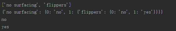
第一节点名为no surfacing,它有两个子节点:一个是名字为0的叶子节点,类标签为no;另一个是名为flippers的判断节点,此处进入递归调用,flippers节点有两个子节点。以前绘制的树形图和此处代表树的数据结构完全相同。
现在我们已经创建了使用决策树的分类器,但是每次使用分类器时,必须重新构造决策树,下面介绍如何在硬盘上存储决策树分类器。
3.2 实用算法:决策树的存储
构造决策树是很耗时的任务,即使处理很小的数据集,如前面的样本数据,也要花费几秒的时间,如果数据集很大,将会耗费很多计算时间。然而用创建好的决策树解决分类问题,则可以很快完成。因此,为了节省计算时间,最好能够在每次执行分类时调用已经构造好的决策树。
为了解决这个问题,需要使用Python模块pickle序列化对象
def storeTree(inputTree, filename):
    import pickle
    fw = open(filename, 'wb')
    pickle.dump(inputTree, fw)  # 将inputTree对象序列化存入已经打开的文件:fw中
    fw.close()


def grabTree(filename):
    import pickle
    fr = open(filename, 'rb')
    return pickle.load(fr)     # 将文件中的对象序列化读出
myTree = treePlotter.retrieveTree(0)
trees.storeTree(myTree,'classifierStorage.txt')
trees.grabTree('classifierStorage.txt')
通过上面的代码,我们可以将分类器存储在硬盘上,而不用每次对数据分类时重新学习一遍,这也是决策树的优点之一。
3.3 示例:使用决策树预测隐形眼镜类型
通过一个例子讲解决策树如何预测患者需要佩戴的隐形眼镜类型。
这里使用的隐形眼镜数据集是非常著名的数据集,它包含很多患者眼部状况的观察条件以及医生推荐的隐形眼镜类型。隐形眼镜类型包括硬材质、软材质以及不适合佩戴隐形眼镜。数据来源于UCI数据库。
import trees
import treePlotter

fr = open('lenses.txt')
lenses = [inst.strip().split('\t') for inst in fr.readlines()]
lensesLables = ['age', 'prescript', 'astigmatic', 'tearRate']
lensesTree = trees.createTree(lenses, lensesLables)
print(lensesTree)
treePlotter.createPlot(lensesTree)
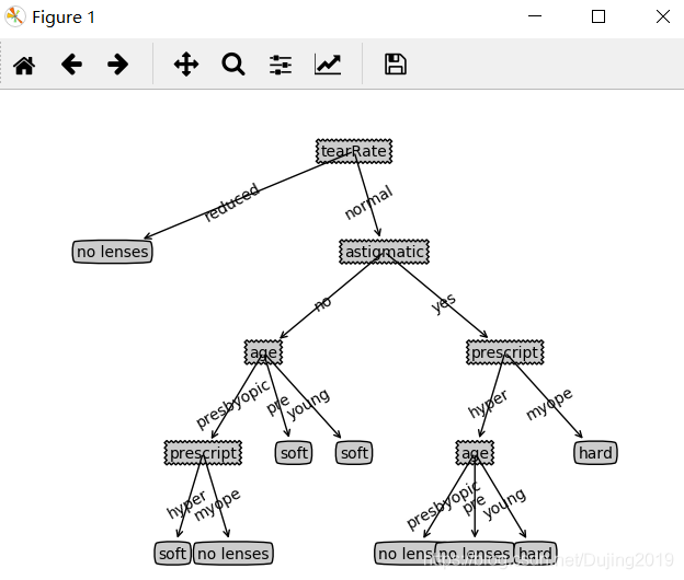
沿着决策树的不同分支,我们可以得到不同患者需要佩戴的隐形眼镜类型。我们也可以发现,医生最多需要问四个问题就能确定患者需要佩戴哪种类型的隐形眼镜。
决策树非常好地匹配了实验数据,然而这些匹配选项可能太多了。将这种问题称之为过度匹配。为了减少过度匹配问题,我们可以裁剪决策树,去掉一些不必要的叶子节点。如果叶子节点只能增加少许信息,则可以删除该节点,将它并入到其他叶子节点中。ID3算法无法直接处理数值型数据,尽管我们可以通过量化的方法将数值型数据转化为标称型数值,但是如果存在太多的特征划分,ID3算法仍然会面临其他问题。
(四)改进算法
4.1 改进ID3算法
下面另外举一个决策树构造实例,验证ID3算法的不足,以及做出新的改进。
数据:14天打球情况
特征:4种环境变化
| outlook | temperature | humidity | windy | play |
|---|---|---|---|---|
| sunny | hot | high | FALSE | no |
| sunny | hot | high | FALSE | no |
| overcast | hot | high | FALSE | yes |
| rainy | mild | high | FALSE | yes |
| rainy | cool | normal | FALSE | yes |
| rainy | cool | normal | TRUE | no |
| overcast | cool | normal | TRUE | yes |
| sunny | mild | high | FALSE | no |
| sunny | cool | normal | FALSE | yes |
| rainy | mild | normal | FALSE | yes |
| sunny | mild | normal | TRUE | yes |
| overcast | mild | high | TRUE | yes |
| overcast | hot | normal | FALSE | yes |
| rainy | mild | high | TRUE | no |
划分方式:4种
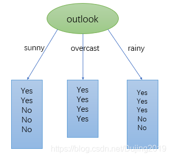
1.基于天气的划分
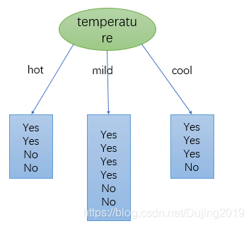
2.基于温度的划分
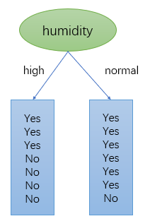
3.基于湿度的划分
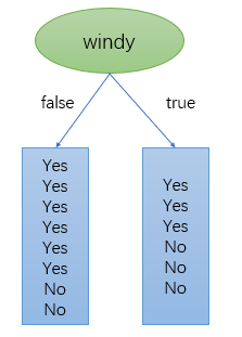
4.基于有风的划分
在历史数据中(14天)有9天打球,5天不打球,所以此时的熵应为:
−
9
14
l
o
g
2
9
14
−
5
14
l
o
g
2
5
14
=
0.940
-\frac{9}{14}log_{2}\frac{9}{14}-\frac{5}{14}log_{2}\frac{5}{14}=0.940
−149log2149−145log2145=0.940
4个特征逐一分析,先从outlook特征开始:
-
当outlook=sunny时,熵值为0.971
( − 2 5 l o g 2 2 5 − 3 5 l o g 2 3 5 = 0.971 ) (-\frac{2}{5}log_{2}\frac{2}{5}-\frac{3}{5}log_{2}\frac{3}{5}=0.971) (−52log252−53log253=0.971) -
当outlook=overcast时,熵值为0
( − 4 4 l o g 2 4 4 = 0 ) (-\frac{4}{4}log_{2}\frac{4}{4}=0) (−44log244=0) -
当outlook=rainy时,熵值为0.971
( − 3 5 l o g 2 3 5 − 2 5 l o g 2 2 5 = 0.971 ) (-\frac{3}{5}log_{2}\frac{3}{5}-\frac{2}{5}log_{2}\frac{2}{5}=0.971) (−53log253−52log252=0.971)
根据数据统计,outlook取值分别为sunny,overcast,rainy的概率分别为: 5/14, 4/14, 5/14
熵值计算:5/14 * 0.971 + 4/14 * 0 + 5/14 * 0.971 = 0.693
信息增益:系统的熵值从原始的0.940下降到了0.693,增益为0.247,信息增益最大,则outlook是根节点。
(gain(temperature)=0.029 gain(humidity)=0.152 gain(windy)=0.048)
同样的方式可以计算出其他特征的信息增益,那么我们选择最大的那个就可以啦,相当于是遍历了一遍特征,找出来根节点,然后再其余的中继续通过信息增益找节点!
现在我们就可以详细分析ID3算法的不足了,假设在outlook特征前面加一个ID特征,ID编号为1到14,在每个节点只有自己一个,那么在1号节点只有一种可能取值,那么熵值就是0,在2号节点只有一种可能取值,那么熵值也是0,以此类推,都是0,加到一起也是0,意味着总体熵值也为0,理想状态下分的特别好的情况才会为0,那么就会误把ID当做根节点,但是把ID当做根节点并没有任何意义。
改进:
C4.5算法:信息增益率(解决ID3问题,考虑自身熵)
ID的信息增益很大,但是对于ID里面的14个特征来说,取到每个特征的概率很小,都是1/14,此时可以看ID自身的熵值
(
(
−
1
14
l
o
g
2
1
14
)
∗
14
)
((-\frac{1}{14}log_{2}\frac{1}{14})*14)
((−141log2141)∗14)
这个值非常大,现在假设信息增益为9,取最大值,但是信息增益率很小:
9
(
−
1
14
l
o
g
2
1
14
)
∗
14
\frac{9}{(-\frac{1}{14}log_{2}\frac{1}{14})*14}
(−141log2141)∗149
这样就解决ID3算法的误差。
CART:使用GINI系数来当做衡量标准
G
i
n
i
(
p
)
=
∑
k
=
1
k
p
k
(
1
−
p
k
)
=
1
−
∑
k
=
1
k
p
k
2
Gini(p)=\sum_{k=1}^{k}p_{k}(1-p_{k})=1-\sum_{k=1}^{k}p_{k}^{2}
Gini(p)=k=1∑kpk(1−pk)=1−k=1∑kpk2
(和熵的衡量标准类似,计算方式不相同)
4.2 决策树剪枝策略
为什么要剪枝:决策树过拟合风险很大,理论上可以完全分得开数据 (想象一下,如果树足够庞大,每个叶子节点不就一个数据了嘛)
剪枝策略:预剪枝,后剪枝
预剪枝:边建立决策树边进行剪枝的操作(更实用),限制深度,叶子节点个数,叶子节点样本数,信息增益量等等。
后剪枝:当建立完决策树后来进行剪枝操作,通过一定的衡量标准:
C
a
(
T
)
=
C
(
T
)
+
α
⋅
∣
T
l
e
a
f
∣
C_{a}(T)=C(T)+\alpha\cdot |T_{leaf}|
Ca(T)=C(T)+α⋅∣Tleaf∣(叶子节点越多,损失越大)
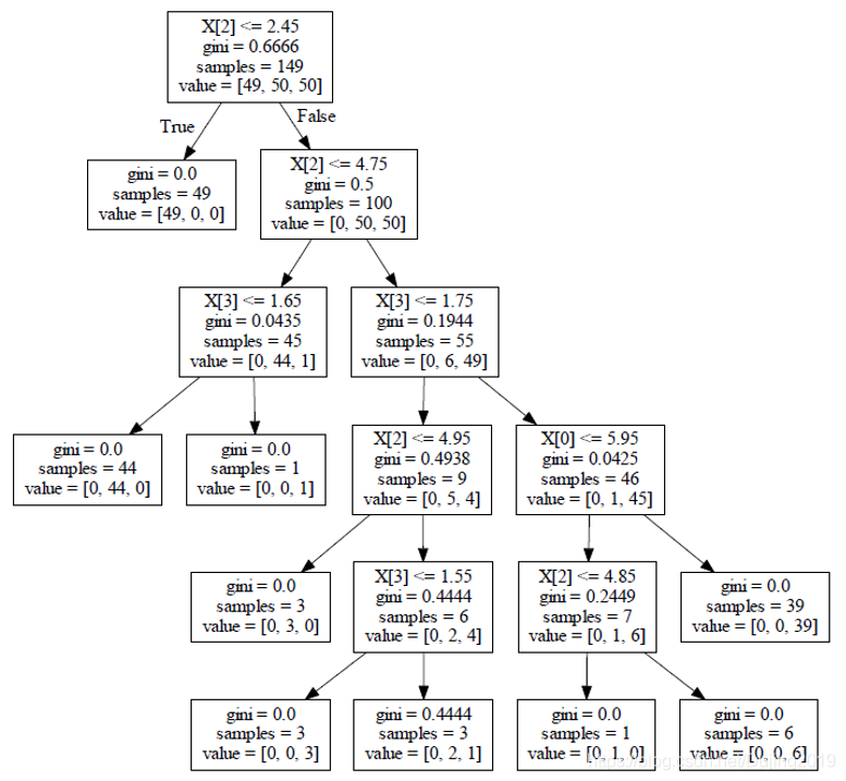
先看根节点。X[2]表示数据集的一个特征,2.45为对于这个特征按照哪个点判断的,0.6666为gini系数,samples表示当前这个节点所有样本个数,value表示这个特征不同类别数量,A类别49个样本,B类别50个样本,C类别50个样本。
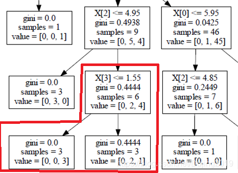
现在观察看这个红色方框,分析X[3]<=1.55这个节点是否需要剪枝。
上面节点的
C
a
(
T
)
C_{a}(T)
Ca(T)值:
0.44
×
6
+
1
⋅
α
0.44\times6+1\cdot\alpha
0.44×6+1⋅α
分裂成下面两个节点的
C
a
(
T
)
C_{a}(T)
Ca(T)值:
0
×
3
+
0.44
×
3
+
2
⋅
α
0\times3+0.44\times3+2\cdot\alpha
0×3+0.44×3+2⋅α
对比两个值的大小,当然这个还取决于 α \alpha α值,具体情况具体分析,选择注重 C ( T ) C(T) C(T)值,还是注重叶子节点数量。 α \alpha α越大,越不过拟合,虽然可能结果没那么好; α \alpha α越小适用于希望结果好,过不过拟合没那么重要的情况。
后剪枝,对比上面两个值,如果剪完后结果小,就剪枝,剪完后损失大,就不剪枝。
(五)决策树实验分析
5.1 树模型可视化展示
import numpy as np
import os
%matplotlib inline
import matplotlib
import matplotlib.pyplot as plt
plt.rcParams['axes.labelsize'] = 14
plt.rcParams['xtick.labelsize'] = 12
plt.rcParams['ytick.labelsize'] = 12
import warnings
warnings.filterwarnings('ignore')
from sklearn.datasets import load_iris
from sklearn.tree import DecisionTreeClassifier

iris = load_iris()
X = iris.data[:,2:]    # petal length and width
y = iris.target

#训练树模型
tree_clf = DecisionTreeClassifier(max_depth=2) #限制树的深度为2
tree_clf.fit(X,y)
DecisionTreeClassifier(class_weight=None, criterion=‘gini’, max_depth=2,
max_features=None, max_leaf_nodes=None,
min_impurity_decrease=0.0, min_impurity_split=None,
min_samples_leaf=1, min_samples_split=2,
min_weight_fraction_leaf=0.0, presort=False, random_state=None,
splitter=‘best’)
from sklearn.tree import export_graphviz
#画图展示
export_graphviz(
    tree_clf,   #树模型
    out_file="iris_tree.dot",
    feature_names=iris.feature_names[2:],
    class_names=iris.target_names,
    rounded=True,
    filled=True
)
可以使用graphviz包中的dot命令行工具将此.dot文件转换为各种格式,如PDF或PNG。下面这条命令行将.dot文件转换为.png图像文件:
$ dot -Tpng iris_tree.dot -o iris_tree.png
from IPython.display import Image
Image(filename='iris_tree.png',width=400,height=400)
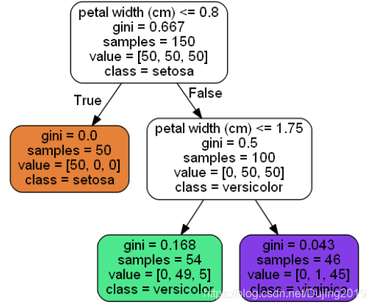
根节点是通过花瓣的宽度判断,是否小于0.8,小于0.8左边,大于0.8右边,根据上面已经解释过这种类型的图,黄色方框表示分配为setosa类型,绿色方框表示分配为versicolor类型,紫色方框表示分配为virginica类型。
5.2 决策树边界展示
from matplotlib.colors import ListedColormap
def plot_decision_boundary(clf, X, y, axes=[0, 7.5, 0, 3], iris=True, legend=False, plot_training=True):
x1s = np.linspace(axes[0], axes[1], 100)
x2s = np.linspace(axes[2], axes[3], 100)
x1, x2 = np.meshgrid(x1s, x2s) #构建棋盘
X_new = np.c_[x1.ravel(), x2.ravel()] #构建测试数据
y_pred = clf.predict(X_new).reshape(x1.shape) #预测最后结果值
custom_cmap = ListedColormap(['#fafab0','#9898ff','#a0faa0'])
plt.contourf(x1, x2, y_pred, alpha=0.3, cmap=custom_cmap)
if not iris:
custom_cmap2 = ListedColormap(['#7d7d58','#4c4c7f','#507d50'])
plt.contour(x1, x2, y_pred, cmap=custom_cmap2, alpha=0.8)
if plot_training:
plt.plot(X[:, 0][y==0], X[:, 1][y==0], "yo", label="Iris-Setosa")
plt.plot(X[:, 0][y==1], X[:, 1][y==1], "bs", label="Iris-Versicolor")
plt.plot(X[:, 0][y==2], X[:, 1][y==2], "g^", label="Iris-Virginica")
plt.axis(axes)
if iris:
plt.xlabel("Petal length", fontsize=14)
plt.ylabel("Petal width", fontsize=14)
else:
plt.xlabel(r"$x_1$", fontsize=18)
plt.ylabel(r"$x_2$", fontsize=18, rotation=0)
if legend:
plt.legend(loc="lower right", fontsize=14)
plt.figure(figsize=(8, 4))
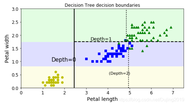
plot_decision_boundary(tree_clf, X, y)
plt.plot([2.45, 2.45], [0, 3], "k-", linewidth=2) #根据上面的图画出每次分裂的位置
plt.plot([2.45, 7.5], [1.75, 1.75], "k--", linewidth=2)
plt.plot([4.95, 4.95], [0, 1.75], "k:", linewidth=2)
plt.plot([4.85, 4.85], [1.75, 3], "k:", linewidth=2)
plt.text(1.40, 1.0, "Depth=0", fontsize=15)
plt.text(3.2, 1.80, "Depth=1", fontsize=13)
plt.text(4.05, 0.5, "(Depth=2)", fontsize=11)
plt.title('Decision Tree decision boundaries')
plt.show()
概率估计
估计类概率输入数据为:花瓣长5厘米,宽1.5厘米的花。 相应的叶节点是深度为2的左节点,因此决策树应输出以下概率:
Iris-Setosa 为 0%(0/54),
Iris-Versicolor 为 90.7%(49/54),
Iris-Virginica 为 9.3%(5/54)。
tree_clf.predict_proba([[5,1.5]]) #预测概率
array([[0. , 0.90740741, 0.09259259]])
tree_clf.predict([[5,1.5]])
array([1])
决策树中的正则化
DecisionTreeClassifier类还有一些其他参数类似地限制了决策树的形状:
- min_samples_split(节点在分割之前必须具有的最小样本数),
- min_samples_leaf(叶子节点必须具有的最小样本数),
- max_leaf_nodes(叶子节点的最大数量),
- max_features(在每个节点处评估用于拆分的最大特征数)。
- max_depth(树最大的深度)
from sklearn.datasets import make_moons
X,y = make_moons(n_samples=100,noise=0.25,random_state=53)
tree_clf1 = DecisionTreeClassifier(random_state=42)
tree_clf2 = DecisionTreeClassifier(min_samples_leaf=4,random_state=42)
tree_clf1.fit(X,y)  #训练
tree_clf2.fit(X,y)

plt.figure(figsize=(12,4))
plt.subplot(121)
plot_decision_boundary(tree_clf1,X,y,axes=[-1.5,2.5,-1,1.5],iris=False)
plt.title('No restrictions')

plt.subplot(122)
plot_decision_boundary(tree_clf2,X,y,axes=[-1.5,2.5,-1,1.5],iris=False)
plt.title('min_samples_leaf=4')
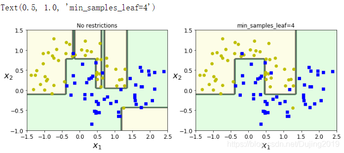
左边不做任何限制,决策边界比较复杂,一些离群点都被捕捉到,为了满足一个样本点,会开扩一个区域;右边指定min_samples_leaf=4,在训练集效果可能不是很好,但是在实际测试上会效果更好一点。
树模型对数据的敏感程度
np.random.seed(6)
Xs = np.random.rand(100, 2) - 0.5
ys = (Xs[:, 0] > 0).astype(np.float32) * 2

angle = np.pi / 4
rotation_matrix = np.array([[np.cos(angle), -np.sin(angle)], [np.sin(angle), np.cos(angle)]])#旋转矩阵
Xsr = Xs.dot(rotation_matrix)#对数据执行旋转

tree_clf_s = DecisionTreeClassifier(random_state=42)
tree_clf_s.fit(Xs, ys)
tree_clf_sr = DecisionTreeClassifier(random_state=42)
tree_clf_sr.fit(Xsr, ys)

plt.figure(figsize=(11, 4))
plt.subplot(121)
plot_decision_boundary(tree_clf_s, Xs, ys, axes=[-0.7, 0.7, -0.7, 0.7], iris=False)
plt.title('Sensitivity to training set rotation')

plt.subplot(122)
plot_decision_boundary(tree_clf_sr, Xsr, ys, axes=[-0.7, 0.7, -0.7, 0.7], iris=False)
plt.title('Sensitivity to training set rotation')

plt.show()
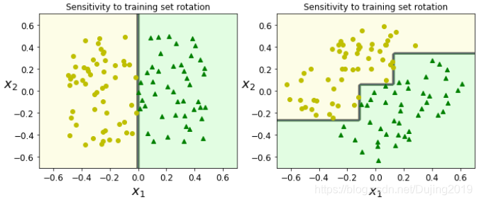
把数据旋转45度,正常会认为决策边界也旋转45度,但是在决策树上不是这个现象,决策树还是会横平竖直切分,树模型对数据的形状是比较敏感的,一旦数据的形状变了,得到的结果也会改变。
5.3 回归任务
决策树不仅能做分类,也能做回归任务。
np.random.seed(42)
m=200
X=np.random.rand(m,1)  #随机选择数据点
y = 4*(X-0.5)**2
y = y + np.random.randn(m,1)/10  #加上随机高斯抖动
from sklearn.tree import DecisionTreeRegressor

tree_reg = DecisionTreeRegressor(max_depth=2)
tree_reg.fit(X,y)
DecisionTreeRegressor(criterion=‘mse’, max_depth=2, max_features=None,
max_leaf_nodes=None, min_impurity_decrease=0.0,
min_impurity_split=None, min_samples_leaf=1,
min_samples_split=2, min_weight_fraction_leaf=0.0,
presort=False, random_state=None, splitter=‘best’)
export_graphviz(
        tree_reg,
        out_file=("regression_tree.dot"),
        feature_names=["x1"],
        rounded=True,
        filled=True
    )
# 第二个决策树
from IPython.display import Image
Image(filename="regression_tree.png",width=400,height=400,)

对比树的深度对结果的影响
from sklearn.tree import DecisionTreeRegressor

tree_reg1 = DecisionTreeRegressor(random_state=42, max_depth=2)  #深度为2
tree_reg2 = DecisionTreeRegressor(random_state=42, max_depth=3)  #深度为3
tree_reg1.fit(X, y)
tree_reg2.fit(X, y)

def plot_regression_predictions(tree_reg, X, y, axes=[0, 1, -0.2, 1], ylabel="$y$"):
    x1 = np.linspace(axes[0], axes[1], 500).reshape(-1, 1)
    y_pred = tree_reg.predict(x1)
    plt.axis(axes)
    plt.xlabel("$x_1$", fontsize=18)
    if ylabel:
        plt.ylabel(ylabel, fontsize=18, rotation=0)
    plt.plot(X, y, "b.")
    plt.plot(x1, y_pred, "r.-", linewidth=2, label=r"$\hat{y}$")

plt.figure(figsize=(11, 4))
plt.subplot(121)

plot_regression_predictions(tree_reg1, X, y)
for split, style in ((0.1973, "k-"), (0.0917, "k--"), (0.7718, "k--")):
    plt.plot([split, split], [-0.2, 1], style, linewidth=2)
plt.text(0.21, 0.65, "Depth=0", fontsize=15)
plt.text(0.01, 0.2, "Depth=1", fontsize=13)
plt.text(0.65, 0.8, "Depth=1", fontsize=13)
plt.legend(loc="upper center", fontsize=18)
plt.title("max_depth=2", fontsize=14)

plt.subplot(122)

plot_regression_predictions(tree_reg2, X, y, ylabel=None)
for split, style in ((0.1973, "k-"), (0.0917, "k--"), (0.7718, "k--")):
    plt.plot([split, split], [-0.2, 1], style, linewidth=2)
for split in (0.0458, 0.1298, 0.2873, 0.9040):
    plt.plot([split, split], [-0.2, 1], "k:", linewidth=1)
plt.text(0.3, 0.5, "Depth=2", fontsize=13)
plt.title("max_depth=3", fontsize=14)

plt.show()
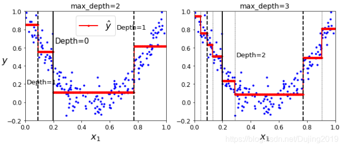
树的深度越多,切分的越细致。看深度得到结果不是很明显,下面还是限制min_samples_leaf:
tree_reg1 = DecisionTreeRegressor(random_state=42)
tree_reg2 = DecisionTreeRegressor(random_state=42, min_samples_leaf=10)
tree_reg1.fit(X, y)
tree_reg2.fit(X, y)

x1 = np.linspace(0, 1, 500).reshape(-1, 1)
y_pred1 = tree_reg1.predict(x1)
y_pred2 = tree_reg2.predict(x1)

plt.figure(figsize=(11, 4))

plt.subplot(121)
plt.plot(X, y, "b.")
plt.plot(x1, y_pred1, "r.-", linewidth=2, label=r"$\hat{y}$")
plt.axis([0, 1, -0.2, 1.1])
plt.xlabel("$x_1$", fontsize=18)
plt.ylabel("$y$", fontsize=18, rotation=0)
plt.legend(loc="upper center", fontsize=18)
plt.title("No restrictions", fontsize=14)

plt.subplot(122)
plt.plot(X, y, "b.")
plt.plot(x1, y_pred2, "r.-", linewidth=2, label=r"$\hat{y}$")
plt.axis([0, 1, -0.2, 1.1])
plt.xlabel("$x_1$", fontsize=18)
plt.title("min_samples_leaf={}".format(tree_reg2.min_samples_leaf), fontsize=14)

plt.show()
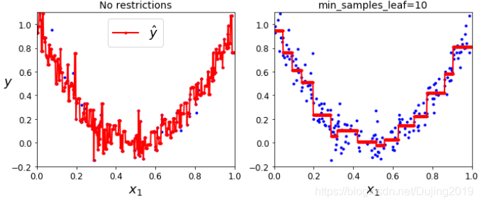
不限制叶子节点必须具有的样本数时,决策树在构建过程中会为了满足每个点,而把决策边界做的非常复杂,而设置限制后,决策边界横平竖直,得到的效果比较好,虽然说也是比较复杂,但是数据本身就是比较复杂的。左边完全过拟合了,右边是规矩的折线。
整体来说,回归做法都是一样的,唯一不同就是建模过程中使用的评估方法不同。
集成算法中也会用到决策树,真正用到决策树,单一的树模型是不够的,以后会学一下集成算法,到时候再写一篇博客吧。


 1万+
1万+


 被折叠的 条评论
为什么被折叠?
被折叠的 条评论
为什么被折叠?
 到【灌水乐园】发言


