机器学习——集成算法

最新推荐文章于 2024-02-17 07:15:00 发布

橘子果酱CV

最新推荐文章于 2024-02-17 07:15:00 发布

阅读量5.5k

点赞数 15

分类专栏：机器学习文章标签： Bagging Boosting Stacking 软投票硬投票

本文链接：https://blog.csdn.net/dujing2019/article/details/98031043

版权

机器学习专栏收录该内容

6 篇文章 5 订阅

订阅专栏

机器学习——集成算法

（一）集成算法原理

集成算法：
构建多个学习器，然后通过一定策略结合把它们来完成学习任务的，常常可以获得比单一学习显著优越的学习器。

集成算法一般分为三类：Bagging，Boosting，Stacking（我们可以把它简单地看成并行，串行和树型）

1.1 Bagging模型

Bagging模型详解

Bagging的全称是bootstrap averaging，它把各个基模型的结果组织起来，具体实现也有很多种类型，以sklearn中提供的Bagging集成算法为例（下面代码中会用到部分算法）：

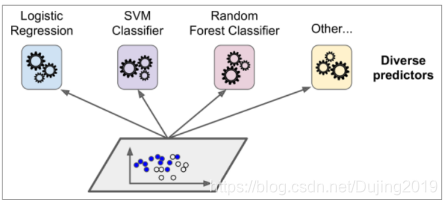
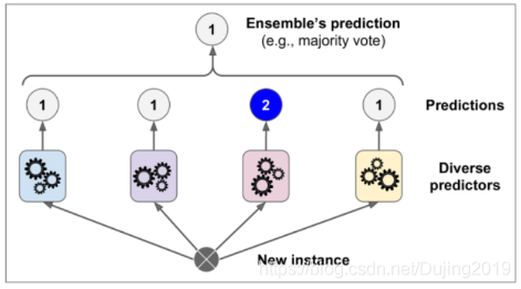
BaggingClassifier/BaggingRegressor是从原始数据集抽选Ｓ次（抽取实例，抽取属性），得到S个新数据集（有的值可能重复，有的值可能不出现）。使用同一模型，训练得到S个分类器，预测时使用投票结果最多的分类。
RandomForestClassifier随机森林，它是对决策树的集成，用随机的方式建立一个决策树的森林。当有一个新的输入样本进入的时候，就让森林中的每一棵决策树分别进行判断，预测时使用投票结果最多的分类，也是少数服从多数的算法。
VotingClassifier，可选择多个不同的基模型，分别进行预测，以投票方式决定最终结果。

Bagging中各个基算法之间没有依赖，可以并行计算，它的结果参考了各种情况，实现的是在欠拟合和过拟合之间取折中。

最典型的代表就是随机森林。

随机：数据采样随机，特征选择随机

森林：很多个决策树并行放在一起

随机森林优势：

它能够处理很高维度（feature很多）的数据，并且不用做特征选择。
在训练完后，它能够给出哪些feature比较重要。
容易做成并行化方法，速度比较快。
可以进行可视化展示，便于分析。

树模型：

理论上越多的树效果会越好，但实际上基本超过一定数量就差不多上下浮动了。

训练多个分类器取平均 $f(x)=1/M\sum_{m=1}^{M}f_{m}(x)$
M表示建立树模型的个数。

1.2 Boosting模型

从弱学习器开始加强，通过加权来进行训练。
$F_{m}(x)=F_{m-1}(x)+argmin_{h}\sum_{i=1}^{n}L(y_{i},F_{m-1}(x_{i}+h(x_{i}))$ （加入一棵树，要比原来强）

一般来说，它的效果会比Bagging好一些。由于新模型是在旧模型的基本上建立的，因此不能使用并行方法训练，并且由于对错误样本的关注，也可能造成过拟合。常见的Boosting算法有：

AdaBoost自适应提升算法，它对分类错误属性的给予更大权重，再做下次迭代，直到收敛。AdaBoost是一个相对简单的Boosting算法，可以自己写代码实现，常见的做法是基模型用单层分类器实现（树桩），桩对应当前最适合划分的属性值位置。
Gradient Boosting Machine（简称GBM）梯度提升算法，它通过求损失函数在梯度方向下降的方法，层层改进，sklearn中也实现了该算法GradientBoostingClassifier/GradientBoostingRegressor。GBM是目前非常流行的一类算法。

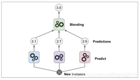
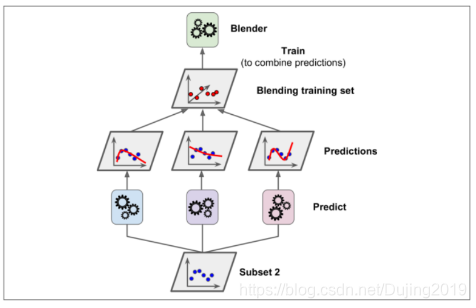
1.3 Stacking模型

聚合多个分类或回归模型（可以分阶段来做)。

Stacking训练一个模型用于组合(combine)其他各个基模型。具体方法是把数据分成两部分，用其中一部分训练几个基模型A1,A2,A3，用另一部分数据测试这几个基模型，把A1,A2,A3的输出作为输入，训练组合模型B。注意，它不是把模型的结果组织起来，而把模型组织起来。理论上，Stacking可以组织任何模型，实际中常使用单层logistic回归作为模型。Sklearn中也实现了stacking模型：StackingClassifier。

（二）集成算法实验分析

集成算法实验分析具体流程见代码注释！！！

集成算法基本思想：

1.训练时用多种分类器一起完成同一份任务

2.测试时对待测试样本分别通过不同的分类器，汇总最后的结果。

2.1 构建实验数据集

import numpy as np
import os
%matplotlib inline
import matplotlib
import matplotlib.pyplot as plt
plt.rcParams['axes.labelsize'] = 14
plt.rcParams['xtick.labelsize'] = 12
plt.rcParams['ytick.labelsize'] = 12
import warnings
warnings.filterwarnings('ignore')
np.random.seed(42)

from sklearn.model_selection import train_test_split
from sklearn.datasets import make_moons

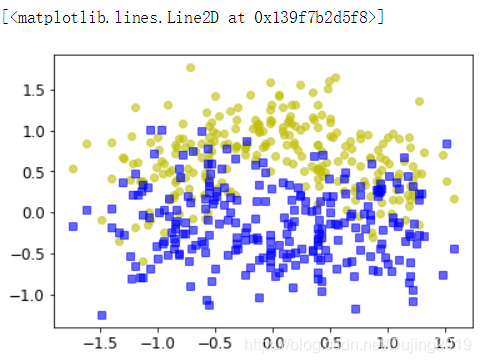
X,y = make_moons(n_samples=500, noise=0.30, random_state=42)   #创建数据集
X_train, X_test, y_train, y_test = train_test_split(X, y, random_state=42)

#绘制数据集图形
plt.plot(X[:,0][y==0],X[:,1][y==0],'yo',alpha = 0.6) #X[:,0][y==0]是0这个类别第一个维度，X[:,1][y==0]是0这个类别第二个维度
plt.plot(X[:,0][y==0],X[:,1][y==1],'bs',alpha = 0.6)

2.2 硬投票和软投票效果

投票策略：软投票与硬投票
硬投票：直接用类别值，少数服从多数。
软投票：各自分类器的概率值进行加权平均

硬投票实验：

from sklearn.ensemble import RandomForestClassifier, VotingClassifier   #随机森林，投票器
from sklearn.linear_model import LogisticRegression  #逻辑回归
from sklearn.svm import SVC   #支持向量机算法

log_clf = LogisticRegression(random_state=42)   #算法实例化 逻辑回归分类器
rnd_clf = RandomForestClassifier(random_state=42)   #随机森林分类器
svm_clf = SVC(random_state=42)   #svc分类器

voting_clf = VotingClassifier(estimators =[('lr',log_clf),('rf',rnd_clf),('svc',svm_clf)],voting='hard')   #构建了投票器使用了所有算法，voting='hard'硬投票

voting_clf.fit(X_train,y_train)  #用当前投票器训练数据

VotingClassifier(estimators=[(‘lr’, LogisticRegression(C=1.0, class_weight=None, dual=False, fit_intercept=True,
intercept_scaling=1, max_iter=100, multi_class=‘warn’,
n_jobs=None, penalty=‘l2’, random_state=42, solver=‘warn’,
tol=0.0001, verbose=0, warm_start=False)), (‘rf’, RandomFore…rbf’, max_iter=-1, probability=False, random_state=42,
shrinking=True, tol=0.001, verbose=False))],
flatten_transform=None, n_jobs=None, voting=‘hard’, weights=None)

from sklearn.metrics import accuracy_score   #准确率
for clf in (log_clf,rnd_clf,svm_clf,voting_clf):  #循环遍历所有算法
    clf.fit(X_train,y_train)
    y_pred = clf.predict(X_test)  #预测测试数据
    print (clf.__class__.__name__,accuracy_score(y_test,y_pred)) #打印名字和准确率

硬投票结果：

LogisticRegression 0.864
RandomForestClassifier 0.872
SVC 0.888
VotingClassifier 0.896

硬投票结果等于0.896，比SVC分类器高出一个百分点，当做集成算法的时候，一般会牺牲一些时间，换来一些准确度或者精度的提升，但是提升不会特别明显，因为提升一个点，本身就不是特别容易，这个集成能够提升一个多点，已经算不错的了。

软投票实验

from sklearn.ensemble import RandomForestClassifier, VotingClassifier   #随机森林，投票器
from sklearn.linear_model import LogisticRegression  #逻辑回归
from sklearn.svm import SVC   #支持向量机算法

log_clf = LogisticRegression(random_state=42)   #算法实例化 逻辑回归分类器
rnd_clf = RandomForestClassifier(random_state=42)   #随机森林分类器
svm_clf = SVC(probability = True,random_state=42)

voting_clf = VotingClassifier(estimators =[('lr',log_clf),('rf',rnd_clf),('svc',svm_clf)],voting='soft')  #软投票

voting_clf.fit(X_train,y_train)

VotingClassifier(estimators=[(‘lr’, LogisticRegression(C=1.0, class_weight=None, dual=False, fit_intercept=True,
intercept_scaling=1, max_iter=100, multi_class=‘warn’,
n_jobs=None, penalty=‘l2’, random_state=42, solver=‘warn’,
tol=0.0001, verbose=0, warm_start=False)), (‘rf’, RandomFore…‘rbf’, max_iter=-1, probability=True, random_state=42,
shrinking=True, tol=0.001, verbose=False))],
flatten_transform=None, n_jobs=None, voting=‘soft’, weights=None)
In [9]:

from sklearn.metrics import accuracy_score   #准确率
for clf in (log_clf,rnd_clf,svm_clf,voting_clf):  #循环遍历所有算法
    clf.fit(X_train,y_train)
    y_pred = clf.predict(X_test)  #预测测试数据
    print (clf.__class__.__name__,accuracy_score(y_test,y_pred)) #打印名字和准确率

LogisticRegression 0.864
RandomForestClassifier 0.872
SVC 0.888
VotingClassifier 0.912

软投票：要求必须各个分别器都能得出概率值，结果比硬投票提升更多的百分点，更靠谱一点。

2.3 Bagging策略效果

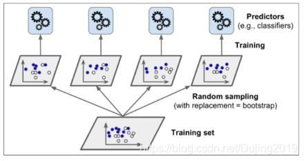
Bagging策略

首先对训练数据集进行多次采样，保证每次得到的采样数据都是不同的。
分别训练多个模型，例如树模型。
预测时需得到所有模型结果再进行集成。

下面做一个对比实验，对比做Bagging与不做Bagging的区别，做一个决策树算法和一个Bagging树，观察它们在决策边界上的差异。

from sklearn.ensemble import BaggingClassifier  #导入Bagging分类器
from sklearn.tree import DecisionTreeClassifier  #导入决策树分类器

bag_clf = BaggingClassifier(DecisionTreeClassifier(),   #基本算法选择树模型
                  n_estimators = 500,   #建立树的数量
                  max_samples = 100,  #最多传进来的样本数
                  bootstrap = True,   #要不要进行一个有放回的随机采样
                  n_jobs = -1,   #要不要做一个多线程，指定-1，就是要
                  random_state = 42  #每次随机策略都是一样的
)
bag_clf.fit(X_train,y_train)  #Bagging分类器训练数据
y_pred = bag_clf.predict(X_test)  #预测

accuracy_score(y_test,y_pred)  #准确率

0.904

#不用Bagging分类器，直接 DecisionTree
tree_clf = DecisionTreeClassifier(random_state = 42)  #树模型实例化，为了保证公平，随机策略都是42
tree_clf.fit(X_train,y_train)
y_pred_tree = tree_clf.predict(X_test)
accuracy_score(y_test,y_pred_tree)

0.856

用 Bagging结果0.904，不用Bagging结果0.856，效果是有提升的，而且提升还比较大。

2.4 集成效果展示分析

集成与传统方法对比

from matplotlib.colors import ListedColormap
def plot_decision_boundary(clf,X,y,axes=[-1.5,2.5,-1,1.5],alpha=0.5,contour =True):  #绘制决策边界
    x1s=np.linspace(axes[0],axes[1],100)    #传入的坐标当做取值范围
    x2s=np.linspace(axes[2],axes[3],100)    
    x1,x2 = np.meshgrid(x1s,x2s)  #合并
    X_new = np.c_[x1.ravel(),x2.ravel()] #坐标棋盘
    y_pred = clf.predict(X_new).reshape(x1.shape)  #得到概率值
    custom_cmap = ListedColormap(['#fafab0','#9898ff','#a0faa0'])
    plt.contourf(x1,x2,y_pred,cmap = custom_cmap,alpha=0.3)
    if contour:
        custom_cmap2 = ListedColormap(['#7d7d58','#4c4c7f','#507d50']) #指定颜色
        plt.contour(x1,x2,y_pred,cmap = custom_cmap2,alpha=0.8)   #绘制等高线
    plt.plot(X[:,0][y==0],X[:,1][y==0],'yo',alpha = 0.6)  #绘制原始数据
    plt.plot(X[:,0][y==0],X[:,1][y==1],'bs',alpha = 0.6)
    plt.axis(axes)
    plt.xlabel('x1')
    plt.xlabel('x2')

plt.figure(figsize = (12,5))
plt.subplot(121)
plot_decision_boundary(tree_clf,X,y) #决策树
plt.title('Decision Tree')
plt.subplot(122)
plot_decision_boundary(bag_clf,X,y)  #集成的Bagging树模型
plt.title('Decision Tree With Bagging')

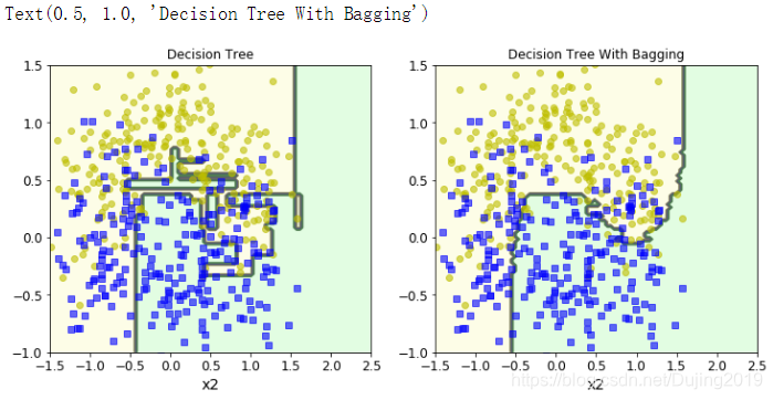
左边展示单用决策树的决策边界，有点杂乱无章，右边是集成后树模型的决策边界，更平稳一些，越平稳的决策边界是我们越想要的，越复杂越乱的决策边界是我们越不想要的。单用决策树，过拟合风险比较大。

2.5 OOB袋外数据的作用

OOB策略(Out Of Bag)

由于随机决策树生成过程采用的Boostrap，所以在一棵树的生成过程并不会使用所有的样本，未使用的样本就叫（Out_of_bag）袋外样本，通过袋外样本，可以评估这个树的准确度，其他子树叶按这个原理评估，最后可以取平均值，即是随机森林算法的性能。

假设现在有100个数据，每次建模都选择了其中80个，那么还有20个就可以直接当做验证集，也就是当我们在建模的时候，自动通过Bagging方法，帮我们把验证集选择出来了。在Bagging模型中，把oob_score 设置为True，可以直接看验证集中的结果，不用额外做一些交叉验证。

bag_clf = BaggingClassifier(DecisionTreeClassifier(),
                  n_estimators = 500,
                  max_samples = 100,
                  bootstrap = True,
                  n_jobs = -1,
                  random_state = 42,
                  oob_score = True
)
bag_clf.fit(X_train,y_train)
bag_clf.oob_score_  #验证的结果

0.9253333333333333

y_pred = bag_clf.predict(X_test)
accuracy_score(y_test,y_pred)  #测试的结果

0.904

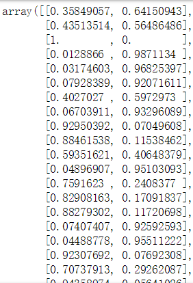
bag_clf.oob_decision_function_  每个样本属于各个类别以及不属于这个类别的概率值

2.6 特征重要性

实例化随机森林，训练数据，展示特征重要性。

from sklearn.ensemble import RandomForestClassifier
rf_clf = RandomForestClassifier() #实例化随机森林分类器
rf_clf.fit(X_train,y_train)  #训练数据

RandomForestClassifier(bootstrap=True, class_weight=None, criterion=‘gini’,
max_depth=None, max_features=‘auto’, max_leaf_nodes=None,
min_impurity_decrease=0.0, min_impurity_split=None,
min_samples_leaf=1, min_samples_split=2,
min_weight_fraction_leaf=0.0, n_estimators=10, n_jobs=None,
oob_score=False, random_state=None, verbose=0,
warm_start=False)

sklearn中是看每个特征的平均深度

from sklearn.datasets import load_iris  #导入数据集
iris = load_iris()   #读取数据
rf_clf = RandomForestClassifier(n_estimators=500,n_jobs=-1)  #树的个数为500个
rf_clf.fit(iris['data'],iris['target'])   #训练数据
for name,score in zip(iris['feature_names'],rf_clf.feature_importances_):   #展示特征重要性
    print (name,score)

sepal length (cm) 0.11105536416721994
sepal width (cm) 0.02319505364393038
petal length (cm) 0.44036215067701534
petal width (cm) 0.42538743151183406

可以看到四个特征的数值都计算出来了，但是看数值特征似乎不太明显，下面分析Mnist数据集中哪些特征比较重要，并用热度图展示。

from sklearn.datasets import fetch_mldata
mnist = fetch_mldata('MNIST original')

rf_clf = RandomForestClassifier(n_estimators=500,n_jobs=-1)  #树的个数为500个
rf_clf.fit(mnist['data'],mnist['target'])  #训练数据

RandomForestClassifier(bootstrap=True, class_weight=None, criterion=‘gini’,
max_depth=None, max_features=‘auto’, max_leaf_nodes=None,
min_impurity_decrease=0.0, min_impurity_split=None,
min_samples_leaf=1, min_samples_split=2,
min_weight_fraction_leaf=0.0, n_estimators=500, n_jobs=-1,
oob_score=False, random_state=None, verbose=0,
warm_start=False)

rf_clf.feature_importances_.shape   #得到特征重要性大小 28x28=784。

(784,)

原始数据有784个像素点，每一个点的特征重要性都能计算出来。

#绘制热度图，显示每一个点的特征重要性
def plot_digit(data):
    image = data.reshape(28,28)
    plt.imshow(image,cmap=matplotlib.cm.hot)
    plt.axis('off')

plot_digit(rf_clf.feature_importances_)  #调用函数
char = plt.colorbar(ticks=[rf_clf.feature_importances_.min(),rf_clf.feature_importances_.max()])   #颜色轴
char.ax.set_yticklabels(['Not important','Very important'])  #指定图中深色浅色的含义

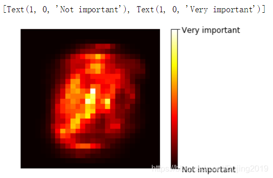
越接近中心，特征重要性越大，越靠近旁边，特征重要性越小，因为mnist 数据集中间是数字，旁边是白边。

2.7 Boosting-提升策略

Bagging相当于并联电路，而Boosting相当于串联电路，先需要做好第一个模型，再做第二个，再做第三个，按照顺序一步一步做。

AdaBoost

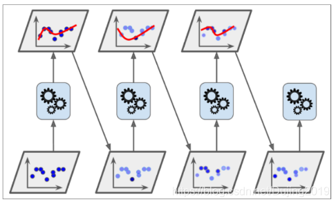
首先拿到数据的时候，所有样本的权重值是一样的，当用一个算法（基本集成算法中都是树模型）进行建模后，发现有的样本拟合的好，有的样本拟合的不好，那么下一个模型要额外注意哪些没拟合好的数据，之前拟合好的数据权重调低一点，没拟合好的数据权重调高一点。再用树模型建立一次，发现可能上一次没做对的样本，在这一次拟合好了，但是又可能出现没有拟合好的样本，那么再调节权重，再次建模，以此类推，最后得到多个基础模型，然后对每个模型加权平均（这个权重是当前模型的表达效果，效果好的权重高点，不好的权重低点）。

以SVM分类器为例来演示AdaBoost的基本策略

from sklearn.svm import SVC

m = len(X_train)   #计算所有样本个数

plt.figure(figsize=(14,5))
for subplot,learning_rate in ((121,1),(122,0.5)):  #不同样本权重调节的力度对结果的影响
    sample_weights = np.ones(m)  #每个样本的权重都设置为一样
    plt.subplot(subplot)
    for i in range(5):  #样本更新五次，得到五个模型，把五个迷行串在一起
        svm_clf = SVC(kernel='rbf',C=0.05,random_state=42)#实例化
        svm_clf.fit(X_train,y_train,sample_weight = sample_weights)   #训练
        y_pred = svm_clf.predict(X_train)  #预测
        sample_weights[y_pred != y_train] *= (1+learning_rate)  #如果y_train与预测值不等，那么就增加权重
        plot_decision_boundary(svm_clf,X,y,alpha=0.2)  #绘制决策边界
        plt.title('learning_rate = {}'.format(learning_rate))
    if subplot == 121:  #在第一幅图的决策边界上标号
        plt.text(-0.7, -0.65, "1", fontsize=14)
        plt.text(-0.6, -0.10, "2", fontsize=14)
        plt.text(-0.5,  0.10, "3", fontsize=14)
        plt.text(-0.4,  0.55, "4", fontsize=14)
        plt.text(-0.3,  0.90, "5", fontsize=14)
plt.show()

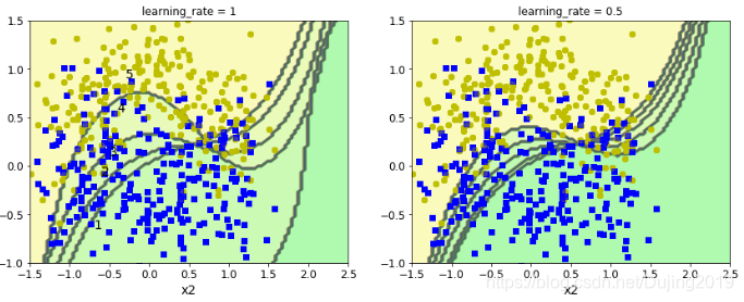
当样本权重越大，变化的趋势也就越大。

from sklearn.ensemble import AdaBoostClassifier
ada_clf = AdaBoostClassifier(DecisionTreeClassifier(max_depth=1),
                   n_estimators = 200,  #更新多少轮
                   learning_rate = 0.5,
                   random_state = 42
)

ada_clf.fit(X_train,y_train)
plot_decision_boundary(ada_clf,X,y)   #绘制决策边界

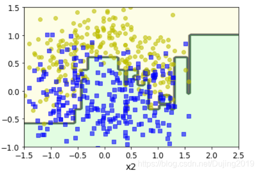
不同的上下梯度就是不同的树模型集成在一起产生的效果。

2.8 GBDT 提升算法流程

np.random.seed(42)
X = np.random.rand(100,1) - 0.5  #构建随机数
y = 3*X[:,0]**2 + 0.05*np.random.randn(100) #对数据点变换

y.shape

(100,)

from sklearn.tree import DecisionTreeRegressor
tree_reg1 = DecisionTreeRegressor(max_depth = 2)   #构建第一棵树
tree_reg1.fit(X,y)  #训练数据

DecisionTreeRegressor(criterion=‘mse’, max_depth=2, max_features=None,
max_leaf_nodes=None, min_impurity_decrease=0.0,
min_impurity_split=None, min_samples_leaf=1,
min_samples_split=2, min_weight_fraction_leaf=0.0,
presort=False, random_state=None, splitter=‘best’)

y2 = y - tree_reg1.predict(X) #查看树中每个样本还差多少没做好
tree_reg2 = DecisionTreeRegressor(max_depth = 2)#构建第二棵树
tree_reg2.fit(X,y2)

DecisionTreeRegressor(criterion=‘mse’, max_depth=2, max_features=None,
max_leaf_nodes=None, min_impurity_decrease=0.0,
min_impurity_split=None, min_samples_leaf=1,
min_samples_split=2, min_weight_fraction_leaf=0.0,
presort=False, random_state=None, splitter=‘best’)

y3 = y2 - tree_reg2.predict(X)  #看第二次结果还有多少没做好
tree_reg3 = DecisionTreeRegressor(max_depth = 2)
tree_reg3.fit(X,y3)

DecisionTreeRegressor(criterion=‘mse’, max_depth=2, max_features=None,
max_leaf_nodes=None, min_impurity_decrease=0.0,
min_impurity_split=None, min_samples_leaf=1,
min_samples_split=2, min_weight_fraction_leaf=0.0,
presort=False, random_state=None, splitter=‘best’)

X_new = np.array([[0.8]])  #测试数据
y_pred = sum(tree.predict(X_new) for tree in (tree_reg1,tree_reg2,tree_reg3))  #预测的结果为三次结果加在一起
y_pred

array([0.75026781])

这就是大致的GBDT算法整个流程。

def plot_predictions(regressors, X, y, axes, label=None, style="r-", data_style="b.", data_label=None):
    x1 = np.linspace(axes[0], axes[1], 500)  #500个数据点
    y_pred = sum(regressor.predict(x1.reshape(-1, 1)) for regressor in regressors)  #当前得到的结果
    plt.plot(X[:, 0], y, data_style, label=data_label) #绘制数据点
    plt.plot(x1, y_pred, style, linewidth=2, label=label)  #绘制曲线
    if label or data_label:
        plt.legend(loc="upper center", fontsize=16)
    plt.axis(axes)

plt.figure(figsize=(11,11))

#展示不同的树，以及树的集成效果。
plt.subplot(321)
plot_predictions([tree_reg1], X, y, axes=[-0.5, 0.5, -0.1, 0.8], label="$h_1(x_1)$", style="g-", data_label="Training set")
plt.ylabel("$y$", fontsize=16, rotation=0)
plt.title("Residuals and tree predictions", fontsize=16)

plt.subplot(322)
plot_predictions([tree_reg1], X, y, axes=[-0.5, 0.5, -0.1, 0.8], label="$h(x_1) = h_1(x_1)$", data_label="Training set")
plt.ylabel("$y$", fontsize=16, rotation=0)
plt.title("Ensemble predictions", fontsize=16)

plt.subplot(323)
plot_predictions([tree_reg2], X, y2, axes=[-0.5, 0.5, -0.5, 0.5], label="$h_2(x_1)$", style="g-", data_style="k+", data_label="Residuals")
plt.ylabel("$y - h_1(x_1)$", fontsize=16)

plt.subplot(324)
plot_predictions([tree_reg1, tree_reg2], X, y, axes=[-0.5, 0.5, -0.1, 0.8], label="$h(x_1) = h_1(x_1) + h_2(x_1)$")
plt.ylabel("$y$", fontsize=16, rotation=0)

plt.subplot(325)
plot_predictions([tree_reg3], X, y3, axes=[-0.5, 0.5, -0.5, 0.5], label="$h_3(x_1)$", style="g-", data_style="k+")
plt.ylabel("$y - h_1(x_1) - h_2(x_1)$", fontsize=16)
plt.xlabel("$x_1$", fontsize=16)

plt.subplot(326)
plot_predictions([tree_reg1, tree_reg2, tree_reg3], X, y, axes=[-0.5, 0.5, -0.1, 0.8], label="$h(x_1) = h_1(x_1) + h_2(x_1) + h_3(x_1)$")
plt.xlabel("$x_1$", fontsize=16)
plt.ylabel("$y$", fontsize=16, rotation=0)

plt.show()

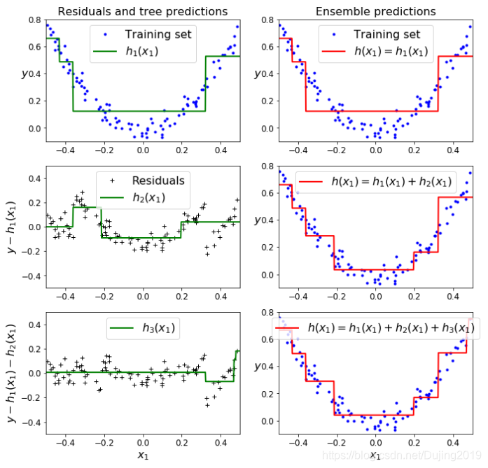
对于第一棵树，左边是单个树（第一幅图），右边是集成（第二幅图），效果是一样的，对于第二棵树（第三幅图），坐标为0的线代表没有残差，0这条直线越往上或者越往下残差越大。把前两棵树集成在一起得到第四幅的结果，可以看到拟合效果变好了，因为第二棵树把第一次没有拟合好的数据点加在一起了。第三棵树（第五幅图）已经越来越往0靠近了，第三次集成（第六幅图）的集成效果差异已经不是特别明显了，也是对数据再进行一次拟合，整个流程就是用相同的模型对数据进行多次集合，在残差上得到的提升。

2.9 集成参数对比分析

from sklearn.ensemble import GradientBoostingRegressor

#实例化
gbrt = GradientBoostingRegressor(max_depth = 2,
                          n_estimators = 3,   #树的数量
                          learning_rate = 1.0, #每个树所占权重
                          random_state = 41
)
gbrt.fit(X,y)

GradientBoostingRegressor(alpha=0.9, criterion=‘friedman_mse’, init=None,
learning_rate=1.0, loss=‘ls’, max_depth=2, max_features=None,
max_leaf_nodes=None, min_impurity_decrease=0.0,
min_impurity_split=None, min_samples_leaf=1,
min_samples_split=2, min_weight_fraction_leaf=0.0,
n_estimators=3, n_iter_no_change=None, presort=‘auto’,
random_state=41, subsample=1.0, tol=0.0001,
validation_fraction=0.1, verbose=0, warm_start=False)

gbrt_slow_1 = GradientBoostingRegressor(max_depth = 2,
                          n_estimators = 3,
                          learning_rate = 0.1,
                          random_state = 41
)
gbrt_slow_1.fit(X,y)

GradientBoostingRegressor(alpha=0.9, criterion=‘friedman_mse’, init=None,
learning_rate=0.1, loss=‘ls’, max_depth=2, max_features=None,
max_leaf_nodes=None, min_impurity_decrease=0.0,
min_impurity_split=None, min_samples_leaf=1,
min_samples_split=2, min_weight_fraction_leaf=0.0,
n_estimators=3, n_iter_no_change=None, presort=‘auto’,
random_state=41, subsample=1.0, tol=0.0001,
validation_fraction=0.1, verbose=0, warm_start=False)

gbrt_slow_1 = GradientBoostingRegressor(max_depth = 2,
                          n_estimators = 3,
                          learning_rate = 0.1,  #改小学习率
                          random_state = 41
)
gbrt_slow_1.fit(X,y)

GradientBoostingRegressor(alpha=0.9, criterion=‘friedman_mse’, init=None,
learning_rate=0.1, loss=‘ls’, max_depth=2, max_features=None,
max_leaf_nodes=None, min_impurity_decrease=0.0,
min_impurity_split=None, min_samples_leaf=1,
min_samples_split=2, min_weight_fraction_leaf=0.0,
n_estimators=3, n_iter_no_change=None, presort=‘auto’,
random_state=41, subsample=1.0, tol=0.0001,
validation_fraction=0.1, verbose=0, warm_start=False)

gbrt_slow_2 = GradientBoostingRegressor(max_depth = 2,
                          n_estimators = 200,  #树的数量调成200个
                          learning_rate = 0.1,
                          random_state = 41
)
gbrt_slow_2.fit(X,y)

GradientBoostingRegressor(alpha=0.9, criterion=‘friedman_mse’, init=None,
learning_rate=0.1, loss=‘ls’, max_depth=2, max_features=None,
max_leaf_nodes=None, min_impurity_decrease=0.0,
min_impurity_split=None, min_samples_leaf=1,
min_samples_split=2, min_weight_fraction_leaf=0.0,
n_estimators=200, n_iter_no_change=None, presort=‘auto’,
random_state=41, subsample=1.0, tol=0.0001,
validation_fraction=0.1, verbose=0, warm_start=False)
In [90]:

plt.figure(figsize = (11,4))
plt.subplot(121)
plot_predictions([gbrt],X,y,axes=[-0.5,0.5,-0.1,0.8],label = 'Ensemble predictions')
plt.title('learning_rate={},n_estimators={}'.format(gbrt.learning_rate,gbrt.n_estimators))

plt.subplot(122)
plot_predictions([gbrt_slow_1],X,y,axes=[-0.5,0.5,-0.1,0.8],label = 'Ensemble predictions')
plt.title('learning_rate={},n_estimators={}'.format(gbrt_slow_1.learning_rate,gbrt_slow_1.n_estimators))

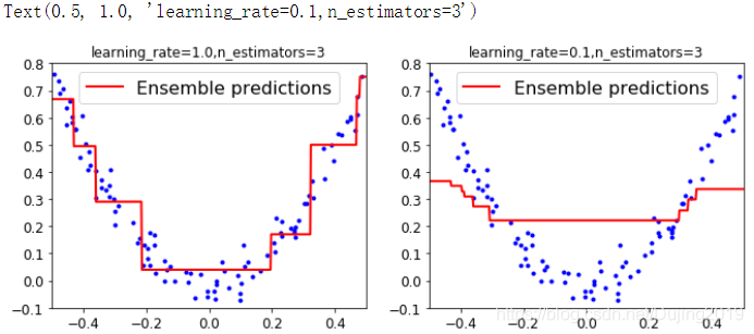
左边是学习率稍微大点的时候，右边是学习率稍微小一点的时候，学习率等于1 的效果比较好，但其实也没有特别好，还是有很多数据点没拟合，所以当学习率比较低的时候，应该增加树的个数，最好在100个以上。

plt.figure(figsize = (11,4))
plt.subplot(121)
plot_predictions([gbrt_slow_2],X,y,axes=[-0.5,0.5,-0.1,0.8],label = 'Ensemble predictions')
plt.title('learning_rate={},n_estimators={}'.format(gbrt_slow_2.learning_rate,gbrt_slow_2.n_estimators))

plt.subplot(122)
plot_predictions([gbrt_slow_1],X,y,axes=[-0.5,0.5,-0.1,0.8],label = 'Ensemble predictions')
plt.title('learning_rate={},n_estimators={}'.format(gbrt_slow_1.learning_rate,gbrt_slow_1.n_estimators))

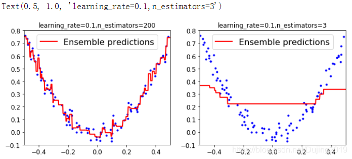
当学习率都为0.1时，可以看到增加了树的数量，效果完全不同，n_estimators等于200的时候，数据点拟合的非常好，n_estimators等于3的时候，大部分数据都没有拟合到。说明在做实验的时候，学习率小一点没关系，但是n_estimators一定要尽可能多一些，100以上最好。

2.10 模型提前停止策略

from sklearn.metrics import mean_squared_error
X_train,X_val,y_train,y_val =  train_test_split(X,y,random_state=49)  #切分数据集
gbrt = GradientBoostingRegressor(max_depth = 2,
                          n_estimators = 120, #树的数量
                          random_state = 42
)
gbrt.fit(X_train,y_train)  #实例化

errors = [mean_squared_error(y_val,y_pred) for y_pred in gbrt.staged_predict(X_val)]   #预测当前回归目标在每个阶段的预测结果的均方误差
bst_n_estimators = np.argmin(errors)  #最好的模型应该是errors 最小的那一次

gbrt_best = GradientBoostingRegressor(max_depth = 2,
                          n_estimators = bst_n_estimators,   #修改迭代次数为最好的迭代次数
                          random_state = 42
) 
  #重新训练
gbrt_best.fit(X_train,y_train)

GradientBoostingRegressor(alpha=0.9, criterion=‘friedman_mse’, init=None,
learning_rate=0.1, loss=‘ls’, max_depth=2, max_features=None,
max_leaf_nodes=None, min_impurity_decrease=0.0,
min_impurity_split=None, min_samples_leaf=1,
min_samples_split=2, min_weight_fraction_leaf=0.0,
n_estimators=55, n_iter_no_change=None, presort=‘auto’,
random_state=42, subsample=1.0, tol=0.0001,
validation_fraction=0.1, verbose=0, warm_start=False)

min_error = np.min(errors)   #打印errors最低的值
min_error

0.002712853325235463

plt.figure(figsize = (11,4))
plt.subplot(121)
plt.plot(errors,'b.-')   #errors曲线
plt.plot([bst_n_estimators,bst_n_estimators],[0,min_error],'k--')   #竖虚线
plt.plot([0,120],[min_error,min_error],'k--')  #横虚线
plt.axis([0,120,0,0.01])  #坐标轴取值范围
plt.title('Val Error')

plt.subplot(122)
plot_predictions([gbrt_best],X,y,axes=[-0.5,0.5,-0.1,0.8])
plt.title('Best Model(%d trees)'%bst_n_estimators)

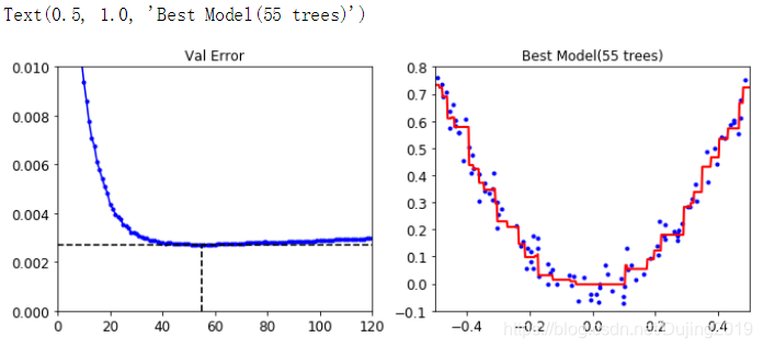
第一幅图是Val Error 随着迭代次数变化的结果，可以看到曲线在变化过程中有回弹趋势，大概在50多次的时候效果最好，第二幅图为最好的那次迭代次数所达到的效果，最好的一次是55棵树，提前停止策略应用场景还是比较广泛的。

gbrt = GradientBoostingRegressor(max_depth = 2,
                             random_state = 42,
                              warm_start =True  #每一次接着之前训练，所以不用设置n_estimators值
)
error_going_up = 0
min_val_error = float('inf')

for n_estimators in range(1,120): 
    gbrt.n_estimators = n_estimators  #动态传入迭代次数
    gbrt.fit(X_train,y_train)  #训练
    y_pred = gbrt.predict(X_val)  #预测
    val_error = mean_squared_error(y_val,y_pred)  #计算error值
    if val_error < min_val_error:    #如果val_error小于最小的val_error
        min_val_error = val_error  #更新min_val_error值
        error_going_up = 0   #计数器
    else:
        error_going_up +=1    #计数器加1
        if error_going_up == 5:  #如果有五次反弹
            break

print (gbrt.n_estimators)  #打印最后一次的迭代次数

61 #因为从55开始。连续迭代五次都是回弹

2.11 Stacking堆叠模型

第一阶段使用不同的分类器得到的几个结果，二阶段会把第一阶段的结果当做输入的特征，最终得到一个结果。

from sklearn.datasets import fetch_mldata
from sklearn.model_selection import train_test_split

mnist = fetch_mldata('MNIST original')  #导入mnist数据集

X_train_val, X_test, y_train_val, y_test = train_test_split(
    mnist.data, mnist.target, test_size=10000, random_state=42)   #数据集切分
X_train, X_val, y_train, y_val = train_test_split(
    X_train_val, y_train_val, test_size=10000, random_state=42)

#选择几种不同的分类器
from sklearn.ensemble import RandomForestClassifier, ExtraTreesClassifier
from sklearn.svm import LinearSVC
from sklearn.neural_network import MLPClassifier

random_forest_clf = RandomForestClassifier(random_state=42)
extra_trees_clf = ExtraTreesClassifier(random_state=42)
svm_clf = LinearSVC(random_state=42)
mlp_clf = MLPClassifier(random_state=42)

estimators = [random_forest_clf, extra_trees_clf, svm_clf, mlp_clf]   #第一阶段选择了四个不同的算法

#分别训练四个分类器
for estimator in estimators:
    print("Training the", estimator)
    estimator.fit(X_train, y_train)

#得到四个分类器的结果
X_val_predictions = np.empty((len(X_val), len(estimators)), dtype=np.float32)

for index, estimator in enumerate(estimators):
    X_val_predictions[:, index] = estimator.predict(X_val)
    
X_val_predictions

array([[2., 2., 2., 2.], #表示第四个分类器都预约是2
[7., 7., 7., 7.],
[4., 4., 4., 4.],
…,
[4., 4., 4., 4.],
[9., 9., 9., 9.],
[4., 4., 4., 4.]], dtype=float32)

#选择随机森林作为二阶段分类器
rnd_forest_blender = RandomForestClassifier(n_estimators=200, oob_score=True, random_state=42)
rnd_forest_blender.fit(X_val_predictions, y_val)

RandomForestClassifier(bootstrap=True, class_weight=None, criterion=‘gini’,
max_depth=None, max_features=‘auto’, max_leaf_nodes=None,
min_impurity_decrease=0.0, min_impurity_split=None,
min_samples_leaf=1, min_samples_split=2,
min_weight_fraction_leaf=0.0, n_estimators=200, n_jobs=None,
oob_score=True, random_state=42, verbose=0, warm_start=False)

rnd_forest_blender.oob_score_  #当前这份数据最终预测结果值

0.9642

橘子果酱CV

关注

15
点赞
踩
42

收藏

觉得还不错? 一键收藏
2
评论
机器学习——集成算法

机器学习——集成算法（一）集成算法原理1.1 Bagging模型1.2 Boosting模型（二）集成算法实验分析2.1 硬投票和软投票效果2.2 OOB袋外数据的作用2.3 特征重要性2.4 Boosting-提升策略（一）集成算法原理目的：让机器学习效果更好，单个不行，集成走起。Bagging：训练多个分类器取平均f(x)=1/M∑m=1Mfm(x)f(x)=1/M\sum_{m=1...
复制链接

扫一扫