cnn应用，接上篇

激活器模块

CNN卷积神经网络并不是只有卷积层，还有采样层和全连接层。在卷积层和全连接层都有激活函数。并且在前向预测和后项传播中需要计算激活函数的前向预测影响，以及误差后项传播影响。所以我们将所有的激活函数形成了一个独立的模块来实现。下面的代码存储为Activators.py

# 1. 当为array的时候，默认d*f就是对应元素的乘积，multiply也是对应元素的乘积，dot（d,f）会转化为矩阵的乘积， dot点乘意味着相加，而multiply只是对应元素相乘，不相加
# 2. 当为mat的时候，默认d*f就是矩阵的乘积，multiply转化为对应元素的乘积，dot（d,f）为矩阵的乘积

import numpy as np

# rule激活器
class ReluActivator(object):
    def forward(self, weighted_input):    # 前向计算，计算输出
        return max(0, weighted_input)

    def backward(self, output):  # 后向计算，计算导数
        return 1 if output > 0 else 0

# IdentityActivator激活器.f(x)=x
class IdentityActivator(object):
    def forward(self, weighted_input):   # 前向计算，计算输出
        return weighted_input

    def backward(self, output):   # 后向计算，计算导数
        return 1

#Sigmoid激活器
class SigmoidActivator(object):
    def forward(self, weighted_input):
        return 1.0 / (1.0 + np.exp(-weighted_input))

    def backward(self, output):
        # return output * (1 - output)
        return np.multiply(output, (1 - output))  # 对应元素相乘

# tanh激活器
class TanhActivator(object):
    def forward(self, weighted_input):
        return 2.0 / (1.0 + np.exp(-2 * weighted_input)) - 1.0

    def backward(self, output):
        return 1 - output * output

# # softmax激活器
# class SoftmaxActivator(object):
#     def forward(self, weighted_input):  # 前向计算，计算输出
#         return max(0, weighted_input)
#
#     def backward(self, output):  # 后向计算，计算导数
#         return 1 if output > 0 else 0

• 1
• 2
• 3
• 4
• 5
• 6
• 7
• 8
• 9
• 10
• 11
• 12
• 13
• 14
• 15
• 16
• 17
• 18
• 19
• 20
• 21
• 22
• 23
• 24
• 25
• 26
• 27
• 28
• 29
• 30
• 31
• 32
• 33
• 34
• 35
• 36
• 37
• 38
• 39
• 40
• 41
• 42
• 43
• 44
• 45
• 46

DNN全连接网络层的实现

将下面的代码存储为DNN.py

# 实现神经网络反向传播算法，以此来训练网络。全连接神经网络可以包含多层，但是只有最后一层输出前有激活函数。
# 所谓向量化编程，就是使用矩阵运算。

import random
import math
import numpy as np
import datetime
import Activators  # 引入激活器模块

# 1. 当为array的时候，默认d*f就是对应元素的乘积，multiply也是对应元素的乘积，dot（d,f）会转化为矩阵的乘积， dot点乘意味着相加，而multiply只是对应元素相乘，不相加
# 2. 当为mat的时候，默认d*f就是矩阵的乘积，multiply转化为对应元素的乘积，dot（d,f）为矩阵的乘积



# 全连接每层的实现类。输入对象x、神经层输出a、输出y均为列向量
class FullConnectedLayer(object):
    # 全连接层构造函数。input_size: 本层输入列向量的维度。output_size: 本层输出列向量的维度。activator: 激活函数
    def __init__(self, input_size, output_size,activator,learning_rate):
        self.input_size = input_size
        self.output_size = output_size
        self.activator = activator
        # 权重数组W。初始化权重为(rand(output_size, input_size) - 0.5) * 2 * sqrt(6 / (output_size + input_size))
        wimin = (output_size - 0.5) * 2 * math.sqrt(6 / (output_size + input_size))
        wimax = (input_size-0.5)*2*math.sqrt(6/(output_size + input_size))
        # self.W = np.random.uniform(wimin,wimax,(output_size, input_size))  #初始化为-0.1~0.1之间的数。权重的大小。行数=输出个数，列数=输入个数。a=w*x，a和x都是列向量
        self.W = np.random.uniform(-0.1, 0.1,(output_size, input_size))  # 初始化为-0.1~0.1之间的数。权重的大小。行数=输出个数，列数=输入个数。a=w*x，a和x都是列向量
        # 偏置项b
        self.b = np.zeros((output_size, 1))  # 全0列向量偏重项
        # 学习速率
        self.learning_rate = learning_rate
        # 输出向量
        self.output = np.zeros((output_size, 1)) #初始化为全0列向量

    # 前向计算，预测输出。input_array: 输入列向量，维度必须等于input_size
    def forward(self, input_array):   # 式2
        self.input = input_array
        self.output = self.activator.forward(np.dot(self.W, input_array) + self.b)

    # 反向计算W和b的梯度。delta_array: 从上一层传递过来的误差项。列向量
    def backward(self, delta_array):
        # 式8
        self.delta = np.multiply(self.activator.backward(self.input),np.dot(self.W.T, delta_array))   #计算当前层的误差，以备上一层使用
        self.W_grad = np.dot(delta_array, self.input.T)   # 计算w的梯度。梯度=误差.*输入
        self.b_grad = delta_array  #计算b的梯度

    # 使用梯度下降算法更新权重
    def update(self):
        self.W += self.learning_rate * self.W_grad
        self.b += self.learning_rate * self.b_grad

• 1
• 2
• 3
• 4
• 5
• 6
• 7
• 8
• 9
• 10
• 11
• 12
• 13
• 14
• 15
• 16
• 17
• 18
• 19
• 20
• 21
• 22
• 23
• 24
• 25
• 26
• 27
• 28
• 29
• 30
• 31
• 32
• 33
• 34
• 35
• 36
• 37
• 38
• 39
• 40
• 41
• 42
• 43
• 44
• 45
• 46
• 47
• 48
• 49
• 50

CNN卷积网络层和Pool降采样层的实现

将下面的代码存储为CNN.py

import numpy as np
import Activators   # 引入自定义的激活器模块
import math

# 获取卷积区域。input_array为单通道或多通道的矩阵顺。i为横向偏移，j为纵向偏移，stride为步幅，filter_width为过滤器宽度，filter_height为过滤器的高度
def get_patch(input_array, i, j, filter_width,filter_height, stride):
    '''
    从输入数组中获取本次卷积的区域，
    自动适配输入为2D和3D的情况
    '''
    start_i = i * stride
    start_j = j * stride
    if input_array.ndim == 2:  #如果只有一个通道
        return input_array[start_i:start_i + filter_height,start_j: start_j + filter_width]
    elif input_array.ndim == 3:  #如果有多个通道，也就是深度上全选
        return input_array[:,start_i: start_i + filter_height,start_j: start_j + filter_width]


# 获取一个2D区域的最大值所在的索引
def get_max_index(array):
    location = np.where(array == np.max(array))
    return location[0], location[1]


# 计算一个过滤器的卷积运算，输出一个二维数据。每个通道的输入是图片，但是可能不是一个通道，所以这里自动适配输入为2D和3D的情况。
def conv(input_array,kernel_array,output_array,stride, bias):
    output_width = output_array.shape[1]   # 获取输出的宽度。一个过滤器产生的输出一定是一个通道
    output_height = output_array.shape[0] # 获取输出的高度
    kernel_width = kernel_array.shape[-1]  # 过滤器的宽度。有可能有多个通道。多通道时shape=[深度、高度、宽度]，单通道时shape=[高度、宽度]
    kernel_height = kernel_array.shape[-2] # 过滤器的高度。有可能有多个通道。多通道时shape=[深度、高度、宽度]，单通道时shape=[高度、宽度]
    for i in range(output_height):
        for j in range(output_width):
            juanjiqu = get_patch(input_array, i, j, kernel_width,kernel_height, stride)   # 获取输入的卷积区。（单通道或多通道）
            # 这里是对每个通道的两个矩阵对应元素相乘求和，再将每个通道的和值求和
            kernel_values= (np.multiply(juanjiqu,kernel_array)).sum() # 卷积区与过滤器卷积运算。1，一个通道内，卷积区矩阵与过滤器矩阵对应点相乘后，求和值。2、将每个通道的和值再求和。
            output_array[i][j] = kernel_values + bias  #将卷积结果加上偏量



# 为数组增加Zero padding。zp步长，自动适配输入为2D和3D的情况
def padding(input_array, zp):
    if zp == 0: # 如果不补0
        return input_array
    else:
        if input_array.ndim == 3:   # 如果输入有多个通道
            input_width = input_array.shape[2]  # 获取输入的宽度
            input_height = input_array.shape[1]  # 获取输入的宽度
            input_depth = input_array.shape[0]  # 获取输入的深度
            padded_array = np.zeros((input_depth,input_height + 2 * zp,input_width + 2 * zp))  # 先定义一个补0后大小的全0矩阵
            padded_array[:,zp: zp + input_height,zp: zp + input_width] = input_array # 每个通道上，将中间部分替换成输入，这样就变成了原矩阵周围补0 的形式
            return padded_array
        elif input_array.ndim == 2:  # 如果输入只有一个通道
            input_width = input_array.shape[1] # 获取输入的宽度
            input_height = input_array.shape[0] # 虎丘输入的高度
            padded_array = np.zeros((input_height + 2 * zp,input_width + 2 * zp))  # 先定义一个补0后大小的全0矩阵
            padded_array[zp: zp + input_height,zp: zp + input_width] = input_array  # 将中间部分替换成输入，这样就变成了原矩阵周围补0 的形式
            return padded_array


# 对numpy数组进行逐个元素的操作。op为函数。element_wise_op函数实现了对numpy数组进行按元素操作，并将返回值写回到数组中
def element_wise_op(array, op):
    for i in np.nditer(array,op_flags=['readwrite']):
        i[...] = op(i)   # 将元素i传入op函数，返回值，再修改i

# Filter类保存了卷积层的参数以及梯度，并且实现了用梯度下降算法来更新参数。
class Filter(object):
    def __init__(self, width, height, depth,filter_num):
        # 卷积核每个元素初始化为[-sqrt(6 / (fan_in + fan_out)), sqrt(6 / (fan_in + fan_out))]。
        # 其中fan_in为输入通道数与滤波器宽高的乘机，即width*height*depth
        # 其中fan_out为输出通道数与滤波器宽高的乘机，即width*height*filter_num
        wimin = -math.sqrt(6 / (width*height*depth + width*height*filter_num))
        wimax = -wimin
        self.weights = np.random.uniform(wimin, wimax, (depth, height, width))  # 随机初始化卷基层权重一个很小的值，
        # self.weights = np.random.uniform(-1e-2, 1e-2,(depth, height, width))  # 随机初始化卷基层权重一个很小的值，
        self.bias = 0  # 初始化偏量为0
        self.weights_grad = np.zeros(self.weights.shape)   # 初始化权重梯度
        self.bias_grad = 0  # 初始化偏量梯度

    def __repr__(self):
        return 'filter weights:\n%s\nbias:\n%s' % (repr(self.weights), repr(self.bias))

    # 读取权重
    def get_weights(self):
        return self.weights

    # 读取偏量
    def get_bias(self):
        return self.bias

    # 更新权重和偏量
    def update(self, learning_rate):
        self.weights -= learning_rate * self.weights_grad
        self.bias -= learning_rate * self.bias_grad

# 用ConvLayer类来实现一个卷积层。下面的代码是初始化一个卷积层，可以在构造函数中设置卷积层的超参数
class ConvLayer(object):
    #初始化构造卷积层：输入宽度、输入高度、通道数、滤波器宽度、滤波器高度、滤波器数目、补零数目、步长、激活器、学习速率
    def __init__(self, input_width, input_height,channel_number, filter_width,filter_height, filter_number,
                 zero_padding, stride, activator,learning_rate):
        self.input_width = input_width   #  输入宽度
        self.input_height = input_height  # 输入高度
        self.channel_number = channel_number  # 通道数=输入的深度=过滤器的深度
        self.filter_width = filter_width  # 过滤器的宽度
        self.filter_height = filter_height  # 过滤器的高度
        self.filter_number = filter_number  # 过滤器的数量。
        self.zero_padding = zero_padding  # 补0圈数
        self.stride = stride # 步幅
        self.output_width = int(ConvLayer.calculate_output_size(self.input_width, filter_width, zero_padding,stride))  # 计算输出宽度
        self.output_height = int(ConvLayer.calculate_output_size(self.input_height, filter_height, zero_padding,stride))  # 计算输出高度
        self.output_array = np.zeros((self.filter_number,self.output_height, self.output_width)) # 创建输出三维数组。每个过滤器都产生一个二维数组的输出
        self.filters = []   # 卷积层的每个过滤器
        for i in range(filter_number):
            self.filters.append(Filter(filter_width,filter_height, self.channel_number,filter_number))
        self.activator = activator   # 使用rule激活器
        self.learning_rate = learning_rate  # 学习速率

    # 计算卷积层的输出。输出结果保存在self.output_array
    def forward(self, input_array):
        self.input_array = input_array  # 多个通道的图片，每个通道为一个二维图片
        self.padded_input_array = padding(input_array,self.zero_padding)  # 先将输入补足0
        for i in range(self.filter_number):  #每个过滤器都产生一个二维数组的输出
            filter = self.filters[i]
            conv(self.padded_input_array,filter.get_weights(), self.output_array[i],self.stride, filter.get_bias())
        # element_wise_op函数实现了对numpy数组进行按元素操作，并将返回值写回到数组中
        element_wise_op(self.output_array,self.activator.forward)

    # 后向传播。input_array为该层的输入，sensitivity_array为当前层的输出误差（和输出的维度相同），activator为激活函数
    def backward(self, input_array, sensitivity_array,activator):

        '''
        计算传递给前一层的误差项，以及计算每个权重的梯度
        前一层的误差项保存在self.delta_array
        梯度保存在Filter对象的weights_grad
        '''

        self.forward(input_array)   # 先根据输入计算经过该卷积层后的输出。（卷积层有几个过滤器，输出层的深度就是多少。输出每一层为一个二维数组）
        self.bp_sensitivity_map(sensitivity_array, activator)   # 将误差传递到前一层，self.delta_array存储上一次层的误差
        self.bp_gradient(sensitivity_array)   # 计算每个过滤器的w和b梯度

    # 按照梯度下降，更新权重
    def update(self):
        for filter in self.filters:
            filter.update(self.learning_rate)   # 每个过滤器


    # 将误差项传递到上一层。sensitivity_array: 本层的误差。activator: 上一层的激活函数
    def bp_sensitivity_map(self, sensitivity_array,activator):   # 公式9
        # 根据卷积步长，对原始sensitivity map进行补0扩展，扩展成如果步长为1的输出误差形状。再用公式8求解
        expanded_error_array = self.expand_sensitivity_map(sensitivity_array)
        # print(sensitivity_array)
        # full卷积，对sensitivitiy map进行zero padding
        # 虽然原始输入的zero padding单元也会获得残差，但这个残差不需要继续向上传递，因此就不计算了
        expanded_width = expanded_error_array.shape[2]   # 误差的宽度
        zp = int((self.input_width + self.filter_width - 1 - expanded_width) / 2)   # 计算步长
        padded_array = padding(expanded_error_array, zp)  #补0操作
        # 初始化delta_array，用于保存传递到上一层的sensitivity map
        self.delta_array = self.create_delta_array()
        # 对于具有多个filter的卷积层来说，最终传递到上一层的sensitivity map相当于所有的filter的sensitivity map之和
        for i in range(self.filter_number):   # 遍历每一个过滤器。每个过滤器都产生多通道的误差，多个多通道的误差叠加
            filter = self.filters[i]
            # 将滤波器每个通道的权重权重翻转180度。
            flipped_weights=[]
            for oneweight in filter.get_weights():  # 这一个滤波器下的每个通道都进行180翻转
                flipped_weights.append(np.rot90(oneweight, 2))
            flipped_weights = np.array(flipped_weights)
            # 计算与一个filter对应的delta_array
            delta_array = self.create_delta_array()
            for d in range(delta_array.shape[0]):   # 计算每个通道上的误差，存储在delta_array的对应通道上
                # print('大小：\n',flipped_weights[d])
                conv(padded_array[i], flipped_weights[d],delta_array[d], 1, 0)
            self.delta_array += delta_array   # 将每个滤波器每个通道产生的误差叠加

        # 将计算结果与激活函数的偏导数做element-wise乘法操作
        derivative_array = np.array(self.input_array)  # 复制一个矩阵，因为下面的会改变元素的值，所以深复制了一个矩阵
        element_wise_op(derivative_array,activator.backward)  # 逐个元素求偏导数。
        self.delta_array *= derivative_array  # 误差乘以偏导数。得到上一层的误差

    # 计算梯度。根据误差值，计算本层每个过滤器的w和b的梯度
    def bp_gradient(self, sensitivity_array):
        # 处理卷积步长，对原始sensitivity map进行扩展，扩展成如果步长为1的输出误差形状。再用公式8求解
        expanded_error_array = self.expand_sensitivity_map(sensitivity_array)
        for i in range(self.filter_number):  # 每个过滤器产生一个输出
            # 计算每个权重的梯度
            filter = self.filters[i]
            for d in range(filter.weights.shape[0]):   # 过滤器的每个通道都要计算梯度
                conv(self.padded_input_array[d],expanded_error_array[i],filter.weights_grad[d], 1, 0)   #  公式（31、32中间）

            # 计算偏置项的梯度
            filter.bias_grad = expanded_error_array[i].sum()   # 公式（34）

    # 对步长为S的sensitivitymap相应的位置进行补0，将其『还原』成步长为1时的sensitivitymap，再用式8进行求解
    def expand_sensitivity_map(self, sensitivity_array):
        depth = sensitivity_array.shape[0]   # 获取误差项的深度
        # 确定扩展后sensitivity map的大小，即计算stride为1时sensitivity map的大小
        expanded_width = (self.input_width - self.filter_width + 2 * self.zero_padding + 1)
        expanded_height = (self.input_height - self.filter_height + 2 * self.zero_padding + 1)
        # 构建新的sensitivity_map
        expand_array = np.zeros((depth, expanded_height, expanded_width))
        # 从原始sensitivity map拷贝误差值，每有拷贝的位置，就是要填充的0
        for i in range(self.output_height):
            for j in range(self.output_width):
                i_pos = i * self.stride
                j_pos = j * self.stride
                expand_array[:, i_pos, j_pos] = sensitivity_array[:, i, j]
        return expand_array

    # 创建用来保存传递到上一层的sensitivity map的数组。（上一层的输出也就是这一层的输入。所以上一层的误差项的维度和这一层的输入的维度相同）
    def create_delta_array(self):
        return np.zeros((self.channel_number,self.input_height, self.input_width))


    # 确定卷积层输出的大小
    @staticmethod
    def calculate_output_size(input_size,filter_size, zero_padding, stride):
        return (input_size - filter_size + 2 * zero_padding) / stride + 1



# Max Pooling层的实现。就是一个卷积区域取最大值，形成输出。除了Max Pooing之外，常用的还有Mean Pooling——取各样本的平均值。
# 采样层并不改变输入的通道数，也不补零，只是通过某种卷积方式实现降采样
class MaxPoolingLayer(object):
    # 构造降采样层，参数为输入宽度、高度、通道数、滤波器宽度、滤波器高度、步长
    def __init__(self, input_width, input_height,channel_number, filter_width,filter_height, stride):
        self.input_width = input_width
        self.input_height = input_height
        self.channel_number = channel_number
        self.filter_width = filter_width
        self.filter_height = filter_height
        self.stride = stride
        self.output_width = int((input_width -filter_width) / self.stride + 1)
        self.output_height = int((input_height -filter_height) / self.stride + 1)
        self.output_array = np.zeros((self.channel_number,self.output_height, self.output_width))

    # 前向计算。
    def forward(self, input_array):
        for d in range(self.channel_number):
            for i in range(self.output_height):
                for j in range(self.output_width):
                    self.output_array[d, i, j] = (get_patch(input_array[d], i, j,self.filter_width,self.filter_height,self.stride).max())   # 获取卷积区后去最大值

    # 后向传播误差
    def backward(self, input_array, sensitivity_array):
        self.delta_array = np.zeros(input_array.shape)
        for d in range(self.channel_number):
            for i in range(self.output_height):
                for j in range(self.output_width):
                    patch_array = get_patch(input_array[d], i, j,self.filter_width,self.filter_height,self.stride)  # 获取卷积区
                    k, l = get_max_index(patch_array)  # 获取最大值的位置
                    self.delta_array[d,i * self.stride + k,j * self.stride + l] = sensitivity_array[d, i, j]   # 更新误差

• 1
• 2
• 3
• 4
• 5
• 6
• 7
• 8
• 9
• 10
• 11
• 12
• 13
• 14
• 15
• 16
• 17
• 18
• 19
• 20
• 21
• 22
• 23
• 24
• 25
• 26
• 27
• 28
• 29
• 30
• 31
• 32
• 33
• 34
• 35
• 36
• 37
• 38
• 39
• 40
• 41
• 42
• 43
• 44
• 45
• 46
• 47
• 48
• 49
• 50
• 51
• 52
• 53
• 54
• 55
• 56
• 57
• 58
• 59
• 60
• 61
• 62
• 63
• 64
• 65
• 66
• 67
• 68
• 69
• 70
• 71
• 72
• 73
• 74
• 75
• 76
• 77
• 78
• 79
• 80
• 81
• 82
• 83
• 84
• 85
• 86
• 87
• 88
• 89
• 90
• 91
• 92
• 93
• 94
• 95
• 96
• 97
• 98
• 99
• 100
• 101
• 102
• 103
• 104
• 105
• 106
• 107
• 108
• 109
• 110
• 111
• 112
• 113
• 114
• 115
• 116
• 117
• 118
• 119
• 120
• 121
• 122
• 123
• 124
• 125
• 126
• 127
• 128
• 129
• 130
• 131
• 132
• 133
• 134
• 135
• 136
• 137
• 138
• 139
• 140
• 141
• 142
• 143
• 144
• 145
• 146
• 147
• 148
• 149
• 150
• 151
• 152
• 153
• 154
• 155
• 156
• 157
• 158
• 159
• 160
• 161
• 162
• 163
• 164
• 165
• 166
• 167
• 168
• 169
• 170
• 171
• 172
• 173
• 174
• 175
• 176
• 177
• 178
• 179
• 180
• 181
• 182
• 183
• 184
• 185
• 186
• 187
• 188
• 189
• 190
• 191
• 192
• 193
• 194
• 195
• 196
• 197
• 198
• 199
• 200
• 201
• 202
• 203
• 204
• 205
• 206
• 207
• 208
• 209
• 210
• 211
• 212
• 213
• 214
• 215
• 216
• 217
• 218
• 219
• 220
• 221
• 222
• 223
• 224
• 225
• 226
• 227
• 228
• 229
• 230
• 231
• 232
• 233
• 234
• 235
• 236
• 237
• 238
• 239
• 240
• 241
• 242
• 243
• 244
• 245
• 246
• 247
• 248
• 249
• 250
• 251
• 252
• 253

CNN识别MNIST数据

有了上面的MNIST数据采集模块，DNN模块，CNN模块，就可以来构建一个包含多层的卷积神经网络实现手写体识别了。

数据集：MNIST数据集，60000张训练图像，10000张测试图像，每张图像size为28*28。每张像素值包含灰度值，即一个0-255之间的整数，而没有rgb三种颜色的值。其实我们可以进一步将像素灰度值，改为黑白像素。每个像素的值为0或1。这样更加方便。

网络层级结构示意图如下：

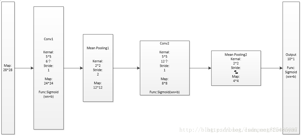
网络层级结构概述：5层神经网络

输入层: 输入数据为原始训练图像（我们在实现中将28*28的灰度图片，改成了28*28的黑白图片）

第一卷积层：6个5*5的过滤器（卷积核），步长Stride为1，不补0，激活函数为sigmoid。在这一层，输入为28*28，深度为1的图片数据，输出为24*24的，深度为6的图片数据。

第一采样层：过滤器（卷积核）为2*2，步长Stride为2。在这一层，输入为24*24的，深度为6的图片数据，输出为12*12的，深度为6的图片数据。

第二卷积层：12个5*5的过滤器（卷积核），步长Stride为1，不补0，激活函数为sigmoid。在这一层，输入为12*12，深度为6的图片数据，输出为8*8的，深度为12的图片数据。

第二采样层：过滤器（卷积核）为2*2，步长Stride为2。在这一层，输入为8*8的，深度为12的图片数据，输出为4*4的，深度为12的图片数据。

输出层：线性函数输入为宽高为（4*4*12，1）的列向量，输出为10维列向量，激活函数为sigmoid。

代码流程概述：

（1）获取训练数据和测试数据；

（2）定义网络层级结构；

（3）初始设置网络参数（权重W，偏向b）

（4）训练网络的超参数的定义（学习率，每次迭代中训练的样本数目，迭代次数）

（5）网络训练——前向运算

（6）网络训练——反向传播

（7）网络训练——参数更新

（8）重复（5）（6）（7），直至满足迭代次数

（9）网络模型测试

# 使用全连接神经网络类，和手写数据加载器，实现验证码识别。

import datetime
import numpy as np
import Activators  # 引入激活器模块
import CNN   # 引入卷积神经网络
import MNIST  # 引入手写数据加载器
import DNN  # 引入全连接神经网络

# 网络模型类
class MNISTNetwork():
    # =============================构造网络结构=============================
    def __init__(self):
        # 初始化构造卷积层：输入宽度、输入高度、通道数、滤波器宽度、滤波器高度、滤波器数目、补零数目、步长、激活器、学习速率
        self.cl1 = CNN.ConvLayer(28, 28, 1, 5, 5, 6, 0, 1, Activators.SigmoidActivator(),0.02)  # 输入28*28 一通道，滤波器5*5的6个，步长为1，不补零，所以输出为24*24深度6
        # 构造降采样层，参数为输入宽度、高度、通道数、滤波器宽度、滤波器高度、步长
        self.pl1 = CNN.MaxPoolingLayer(24, 24, 6, 2, 2, 2)  # 输入24*24，6通道，滤波器2*2，步长为2，所以输出为12*12，深度保持不变为6
        # 初始化构造卷积层：输入宽度、输入高度、通道数、滤波器宽度、滤波器高度、滤波器数目、补零数目、步长、激活器、学习速率
        self.cl2 = CNN.ConvLayer(12, 12, 6, 5, 5, 12, 0, 1, Activators.SigmoidActivator(),0.02)  # 输入12*12，6通道，滤波器5*5的12个，步长为1，不补零，所以输出为8*8深度12
        # 构造降采样层，参数为输入宽度、高度、通道数、滤波器宽度、滤波器高度、步长
        self.pl2 = CNN.MaxPoolingLayer(8, 8, 12, 2, 2, 2)  # 输入8*8，12通道，滤波器2*2，步长为2，所以输出为4*4，深度保持不变为12。共192个像素
        # 全连接层构造函数。input_size: 本层输入向量的维度。output_size: 本层输出向量的维度。activator: 激活函数
        self.fl1 = DNN.FullConnectedLayer(192, 10, Activators.SigmoidActivator(),0.02)  # 输入192个像素，输出为10种分类概率,学习速率为0.05

    # 根据输入计算一次输出。因为卷积层要求的数据要求有通道数，所以onepic是一个包含深度，高度，宽度的多维矩阵
    def forward(self,onepic):
        # print('图片：',onepic.shape)
        self.cl1.forward(onepic)
        # print('第一层卷积结果：',self.cl1.output_array.shape)
        self.pl1.forward(self.cl1.output_array)
        # print('第一层采样结果：',self.pl1.output_array.shape)
        self.cl2.forward(self.pl1.output_array)
        # print('第二层卷积结果：',self.cl2.output_array.shape)
        self.pl2.forward(self.cl2.output_array)
        # print('第二层采样结果：',self.pl2.output_array.shape)
        flinput = self.pl2.output_array.flatten().reshape(-1, 1)  # 转化为列向量
        self.fl1.forward(flinput)
        # print('全连接层结果：',self.fl1.output.shape)
        return  self.fl1.output

    def backward(self,onepic,labels):
        # 计算误差
        delta = np.multiply(self.fl1.activator.backward(self.fl1.output), (labels - self.fl1.output))  # 计算输出层激活函数前的误差
        # print('输出误差：',delta.shape)

        # 反向传播
        self.fl1.backward(delta)  # 计算了全连接层输入前的误差，以及全连接的w和b的梯度
        self.fl1.update()  # 更新权重w和偏量b
        # print('全连接层输入误差：', self.fl1.delta.shape)
        sensitivity_array = self.fl1.delta.reshape(self.pl2.output_array.shape)  # 将误差转化为同等形状
        self.pl2.backward(self.cl2.output_array, sensitivity_array)  # 计算第二采样层的输入误差。参数为第二采样层的 1、输入，2、输出误差
        # print('第二采样层的输入误差：', self.pl2.delta_array.shape)
        self.cl2.backward(self.pl1.output_array, self.pl2.delta_array,Activators.SigmoidActivator())  # 计算第二卷积层的输入误差。参数为第二卷积层的 1、输入，2、输出误差，3、激活函数
        self.cl2.update()  # 更新权重w和偏量b
        # print('第二卷积层的输入误差：', self.cl2.delta_array.shape)
        self.pl1.backward(self.cl1.output_array, self.cl2.delta_array)  # 计算第一采样层的输入误差。参数为第一采样层的 1、输入，2、输出误差
        # print('第一采样层的输入误差：', self.pl1.delta_array.shape)
        self.cl1.backward(onepic, self.pl1.delta_array,Activators.SigmoidActivator())  # 计算第一卷积层的输入误差。参数为第一卷积层的 1、输入，2、输出误差，3、激活函数
        self.cl1.update()  # 更新权重w和偏量b
        # print('第一卷积层的输入误差：', self.cl1.delta_array.shape)



# 由于使用了逻辑回归函数，所以只能进行分类识别。识别ont-hot编码的结果
if __name__ == '__main__':

    # =============================加载数据集=============================
    train_data_set, train_labels = MNIST.get_training_data_set(60000, False)  # 加载训练样本数据集，和one-hot编码后的样本标签数据集
    test_data_set, test_labels = MNIST.get_test_data_set(10000, False)  # 加载测试特征数据集，和one-hot编码后的测试标签数据集
    train_data_set = np.array(train_data_set).astype(bool).astype(int)    #可以将图片简化为黑白图片
    train_labels = np.array(train_labels)
    test_data_set = np.array(test_data_set).astype(bool).astype(int)    #可以将图片简化为黑白图片
    test_labels = np.array(test_labels)
    print('样本数据集的个数：%d' % len(train_data_set))
    print('测试数据集的个数：%d' % len(test_data_set))


    # =============================构造网络结构=============================
    mynetwork =MNISTNetwork()

    # 打印输出每层网络
    # print('第一卷积层：\n',mynetwork.cl1.filters)
    # print('第二卷积层：\n', mynetwork.cl2.filters)
    # print('全连接层w：\n', mynetwork.fl1.W)
    # print('全连接层b：\n', mynetwork.fl1.b)

    # =============================迭代训练=============================
    for i in range(20):  #迭代训练10次。每个迭代内，对所有训练数据进行训练，更新（训练图像个数/batchsize）次网络参数
        print('迭代：',i)
        for k in range(train_data_set.shape[0]):  #使用每一个样本进行训练
            # 正向计算
            onepic =train_data_set[k]
            onepic = np.array([onepic])  # 卷积神经网络要求的输入必须包含深度、高度、宽度三个维度。
            result = mynetwork.forward(onepic)   # 前向计算一次
            # print(result.flatten())
            labels = train_labels[k].reshape(-1, 1)  # 获取样本输出，转化为列向量
            mynetwork.backward(onepic,labels)



    # 打印输出每层网络
    # print('第一卷积层：\n',mynetwork.cl1.filters)
    # print('第二卷积层：\n', mynetwork.cl2.filters)
    # print('全连接层w：\n', mynetwork.fl1.W)
    # print('全连接层b：\n', mynetwork.fl1.b)

    # =============================评估结果=============================
    right = 0
    for k in range(train_data_set.shape[0]):  # 使用每一个样本进行训练
        # 正向计算
        onepic = train_data_set[k]
        onepic = np.array([onepic])  # 卷积神经网络要求的输入必须包含深度、高度、宽度三个维度。
        result = mynetwork.forward(onepic)  # 前向计算一次
        labels = train_labels[k].reshape(-1, 1)  # 获取样本输出，转化为列向量
        # print(result)
        pred_type = result.argmax()
        real_type = labels.argmax()

        # print(pred_type,real_type)
        if pred_type==real_type:
            right+=1

    print('%s after right ratio is %f' % (datetime.datetime.now(), right/test_data_set.shape[0]))  # 打印输出错误率

• 1
• 2
• 3
• 4
• 5
• 6
• 7
• 8
• 9
• 10
• 11
• 12
• 13
• 14
• 15
• 16
• 17
• 18
• 19
• 20
• 21
• 22
• 23
• 24
• 25
• 26
• 27
• 28
• 29
• 30
• 31
• 32
• 33
• 34
• 35
• 36
• 37
• 38
• 39
• 40
• 41
• 42
• 43
• 44
• 45
• 46
• 47
• 48
• 49
• 50
• 51
• 52
• 53
• 54
• 55
• 56
• 57
• 58
• 59
• 60
• 61
• 62
• 63
• 64
• 65
• 66
• 67
• 68
• 69
• 70
• 71
• 72
• 73
• 74
• 75
• 76
• 77
• 78
• 79
• 80
• 81
• 82
• 83
• 84
• 85
• 86
• 87
• 88
• 89
• 90
• 91
• 92
• 93
• 94
• 95
• 96
• 97
• 98
• 99
• 100
• 101
• 102
• 103
• 104
• 105
• 106
• 107
• 108
• 109
• 110
• 111
• 112
• 113
• 114
• 115
• 116
• 117
• 118
• 119
• 120
• 121
• 122
• 123
• 124