EfficientNet的解读与Tensorflow 2.0实现

EfficientNet论文解读

Efficient Net是Google在2019年发表的一篇论文，系统的研究了如何在给定资源的条件下，如何平衡扩展网络的深度，广度以及图像的分辨率这三者的关系，来取得最好的图像识别精度。作者提出了一种新的方法来统一的扩展这几个维度，并在Resnet和Mobilenet的基础上验证了这种方法的有效性。

作者首先用NAS（神经网络搜索）的方法来设计一个基准网络EfficientNet-B0，然后在这个模型之上进行扩展，得到一系列的模型，其中的EfficientNet-B7在Imagenet上获得了84.4% Top1和97.5 Top5的分类准确率，是迄今为止的最好结果，同时该模型相比以前的最好的卷积网络，模型参数小了8.4倍，运行速度快了6.1倍。

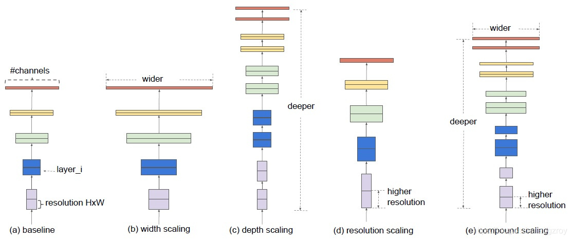
在以前的研究中可以看到，对卷积网络进行扩展可以获得更好的性能，例如Resnet扩展了网络的深度，从18层扩展到200层，或者可以对网络的宽度进行扩展（增加Filters)，以及比较少见的扩展网络输入图片的分辨率。但是之前的研究只是关注在扩展深度，宽度，分辨率这三者之一，如果要同时扩展这三者，则通常需要手工进行繁琐的网络优化，而效果也并不理想。下图是网络扩展的几种形式：

下图是分别对同一个基准网络单独进行深度，宽度，图像分辨率扩展所带来的性能提升：

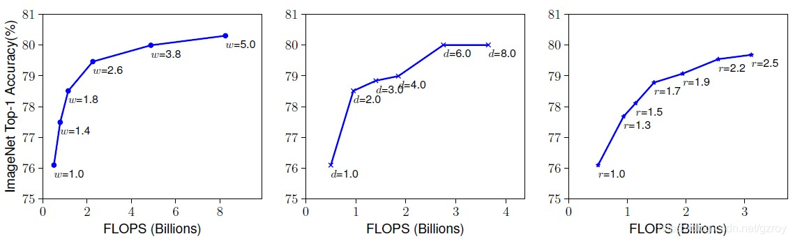
从上图可以看到，随着网络的扩展，运算量增加，网络的性能也随着提升，但是扩展到一定程度之后网络的性能出现饱和，即网络的扩展无法带来相应的性能提升。这也是作者得到的第一个观察结论。

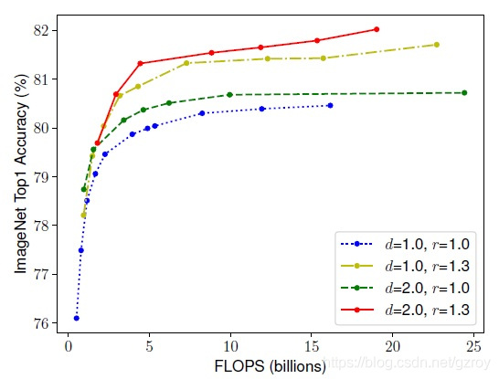
从经验可得，不同维度的扩展并不是独立的。直觉上，对于高分辨率的图像，我们需要增加网络的深度以获得对较大图像的大的感受野，同样我们也需要增加网络的宽度与以便更好的捕捉个高分辨率图像下的像素模式。因此我们需要协调和平衡这几个维度的扩展。这是作者得到的第二个观察结论。

下图是同时扩展网络的深度，宽度和分辨率所观察到的基准网络的性能提升。

作者在论文中提出了一种新的复合扩展方法，采用了一个复合扩展系数Φ来统一扩展网络的深度，宽度和分辨率，如下所示：

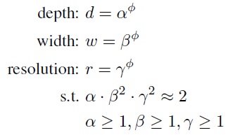
其中α,β,γ是通过网格搜索得出的常数，Φ是用户指定的一个系数，用于控制有多少资源可用于模型的扩展，同时α,β,γ指定如何分配这些资源给到模型的深度，宽度和分辨率扩展之用。对于卷积网络的计算量FLOPS来说，是和网络的d,w^2,r^2成比例的。即增大2倍网络的深度需要2倍的FLOPS，但是增大2倍的宽度需要4倍的FLOPS。

作者采用NAS搜索的方式设计了一个有效的基准网络，命名为EfficientNet-B0，网络的结构如下：

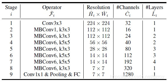
这个网络结构和Mnas-net非常相似。里面的基本结构是Inverted bottleneck MBConv，另外这个MBConv的Block还增加了Squeeze-Excitation模块。具体介绍可以参加Mans-net以及mobilenet V2这两篇论文。

基于这个基准模型，作者通过以下2个步骤来应用之前提到的复合扩展方法。

步骤1：固定Φ=1，假设有2倍的资源可用，通过网格搜索来确定α,β,γ。最终结论是对于EfficientNet-B0，在满足约束α×β^2×γ^2≈2的条件下，α,β,γ的最佳数值是α=1.1，β=1.1，γ=1.15

步骤2：按照步骤1得出的α,β,γ的值，设定不同的Φ（2-7）来扩展基准模型，最终得到EfficientNet-B1到B7的网络结构。

从作者给出的官方代码中，我们可以更加详细的看到EfficientNet B0-B7之间的各维度的扩展情况：

params_dict = {
      # (width_coefficient, depth_coefficient, resolution, dropout_rate)
      'efficientnet-b0': (1.0, 1.0, 224, 0.2),
      'efficientnet-b1': (1.0, 1.1, 240, 0.2),
      'efficientnet-b2': (1.1, 1.2, 260, 0.3),
      'efficientnet-b3': (1.2, 1.4, 300, 0.3),
      'efficientnet-b4': (1.4, 1.8, 380, 0.4),
      'efficientnet-b5': (1.6, 2.2, 456, 0.4),
      'efficientnet-b6': (1.8, 2.6, 528, 0.5),
      'efficientnet-b7': (2.0, 3.1, 600, 0.5),
      'efficientnet-b8': (2.2, 3.6, 672, 0.5),
      'efficientnet-l2': (4.3, 5.3, 800, 0.5),
  }

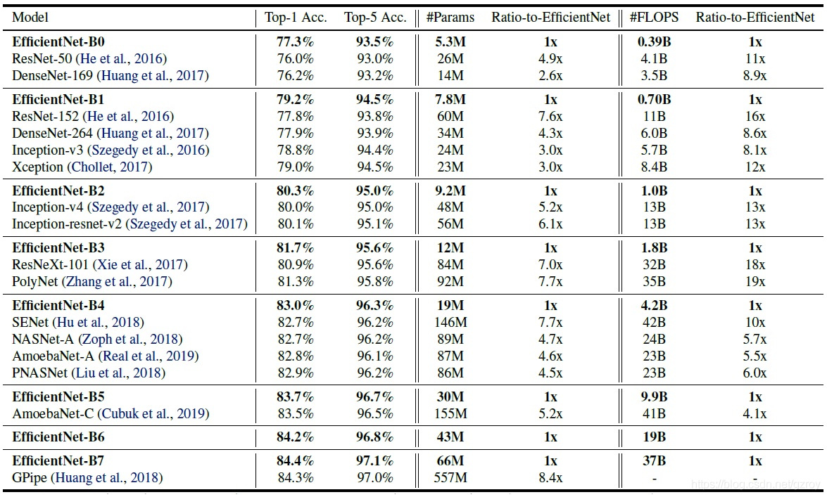
下表是EfficientNet B0-B7的性能以及和其他网络模型的对比，可以看到在实现相近的精度的条件下，EfficientNet比其他的网络模型所需要的FLOPS大大减少，从而带来了Inference阶段的速度的提升：

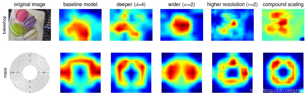
为了更好的理解复合扩展是如何带来精度的提升，作者还比较了不同的扩展条件下的激活图(class activation map)，如下图所示，可以看到，复合扩展的模型更好的关注到了和图像的细节相关的区域。

Tensorflow 2.0实现

作者提供了Tensorflow的官方代码，https://github.com/tensorflow/tpu/tree/master/models/official/efficientnet

不过我看了一下代码，写得比较复杂，有些细节在论文里面没有描述到，例如代码里面的superpixel_kernel，因此我尝试基于Tensorflow 2.0做一个简洁的复现。

首先我们构建一个efficientnet的模型，定义在efficientnet.py文件中，代码如下：

import tensorflow as tf
import math
l = tf.keras.layers
se_ratio = 0.25
weight_decay = 1e-5
def _conv(inputs, filters, kernel_size, strides, bias=False, normalize=True, activation='swish'):
    output = inputs
    padding_str = 'same'
    output = l.Conv2D(
        filters, kernel_size, strides, padding_str, use_bias=bias, \
        kernel_initializer='he_normal', data_format='channels_first', \
        kernel_regularizer=tf.keras.regularizers.l2(l=weight_decay)
    )(output)
    if normalize:
        output = l.BatchNormalization(axis=1)(output)
    if activation=='relu':
        output = l.ReLU()(output)
    if activation=='relu6':
        output = l.ReLU(max_value=6)(output)
    if activation=='leaky_relu':
        output = l.LeakyReLU(alpha=0.1)(output)
    if activation=='sigmoid':
        output = l.Activation('sigmoid')(output)
    if activation=='swish':
        output = l.Activation(tf.nn.swish)(output)
    return output
 
def _dwconv(inputs, kernel_size, strides, bias=True, activation='swish'):
    output = inputs
    padding_str = 'same'
    output = l.DepthwiseConv2D(
        kernel_size, strides, padding_str, use_bias=bias, data_format='channels_first', \
        depthwise_initializer='he_uniform', depthwise_regularizer=tf.keras.regularizers.l2(l=weight_decay))(output)
    output = l.BatchNormalization(axis=1)(output)
    if activation=='relu':
        output = l.ReLU()(output)
    if activation=='relu6':
        output = l.ReLU(max_value=6)(output)
    if activation=='leaky_relu':
        output = l.LeakyReLU(alpha=0.1)(output)
    if activation=='swish':
        output = l.Activation(tf.nn.swish)(output)
    return output
 
def _bottleneck(inputs, in_filters, out_filters, kernel_size, strides, bias=False, activation='swish', t=1):
    output = _conv(inputs, in_filters*t, 1, 1, False, True, activation)
    output = _dwconv(output, kernel_size, strides, False, activation)
    #SE Layer
    se_output = tf.reduce_mean(output, axis=[2,3], keepdims=True)
    squeeze_filter = max(1, int(in_filters*se_ratio))
    se_output = _conv(se_output, squeeze_filter, 1, 1, True, False, activation)
    se_output = _conv(se_output, in_filters*t, 1, 1, True, False, 'sigmoid')
    output = se_output*output
    #Conv
    output = _conv(output, out_filters, 1, 1, False, True, 'linear')
    if strides==1 and in_filters==out_filters:
        output = l.add([output, inputs])
    return output

def _block(inputs, in_filters, out_filters, kernel_size, strides, bias=False, activation='swish', t=1, repeats=1):
    output = _bottleneck(inputs, in_filters, out_filters, kernel_size, strides, bias, activation, t)
    for i in range(repeats-1):
        output = _bottleneck(output, out_filters, out_filters, kernel_size, 1, bias, activation, t)
    return output

def round_filters(filters, beta):
    divisor = 8
    filters *= beta
    new_filters = max(divisor, int(filters + divisor / 2) // divisor * divisor)
    # Make sure that round down does not go down by more than 10%.
    if new_filters < 0.9 * filters:
        new_filters += divisor
    return int(new_filters)

def round_repeats(repeats, alpha):
    return int(math.ceil(alpha * repeats))
 
def efficientnet_model(alpha,beta,gamma,dropout):
    # Input Layer
    image = tf.keras.Input(shape=(3,None,None))                        #224*224*3
    out_filter = round_filters(32, beta)
    net = _conv(image, out_filter, 3, 2, False, True, 'swish')            #112*112*32
    #MBConv Block 1
    repeats = round_repeats(1, alpha)
    in_filter = round_filters(32, beta)
    out_filter = round_filters(16, beta)
    net = _block(net, in_filter, out_filter, 3, 1, False, 'swish', 1, repeats)    #112*112*16
    #MBConv Block 2
    repeats = round_repeats(2, alpha)
    in_filter = round_filters(16, beta)
    out_filter = round_filters(24, beta)
    net = _block(net, in_filter, out_filter, 3, 2, False, 'swish', 6, repeats)    #56*56*24
    #MBConv Block 3
    repeats = round_repeats(2, alpha)
    in_filter = round_filters(24, beta)
    out_filter = round_filters(40, beta)
    net = _block(net, in_filter, out_filter, 5, 2, False, 'swish', 6, repeats)    #28*28*40
    #MBConv Block 4
    repeats = round_repeats(3, alpha)
    in_filter = round_filters(40, beta)
    out_filter = round_filters(80, beta)
    net = _block(net, in_filter, out_filter, 3, 2, False, 'swish', 6, repeats)    #14*14*80
    #MBConv Block 5
    repeats = round_repeats(3, alpha)
    in_filter = round_filters(80, beta)
    out_filter = round_filters(112, beta)
    net = _block(net, in_filter, out_filter, 5, 1, False, 'swish', 6, repeats)    #14*14*112
    #MBConv Block 6
    repeats = round_repeats(4, alpha)
    in_filter = round_filters(112, beta)
    out_filter = round_filters(192, beta)
    net = _block(net, in_filter, out_filter, 5, 2, False, 'swish', 6, repeats)    #7*7*192
    #MBConv Block 7
    repeats = round_repeats(1, alpha)
    in_filter = round_filters(192, beta)
    out_filter = round_filters(320, beta)
    net = _block(net, in_filter, out_filter, 3, 1, False, 'swish', 6, repeats)    #7*7*320
    #Conv
    out_filter = round_filters(1280, beta)
    net = _conv(net, out_filter, 1, 1, False, True, 'swish')            #7*7*1280
    net = tf.reduce_mean(net, axis=[2,3], keepdims=False)                 #GlobalPool, 1280
    net = l.Dropout(rate=dropout)(net)
    logits = l.Dense(units=1000, name='output')(net)
    model = tf.keras.Model(inputs=image, outputs=logits)
    return model 

在构建efficientnet模型时，需要传入alpha, beta, gamma，dropout这4个参数，其中alpha, beta, gamma对应的是论文中提到的深度，宽度，分辨率这三个维度的扩展系数，当这3个参数都取1.0时，对应的是efficientnet-B0这个模型。

之后我们就可以调用这个模型来进行Imagenet的训练了，代码分为以下几部分：

1. 定义相关的参数。

import tensorflow as tf
import tensorflow_addons as tfa
import math
import os
import random
import time
import numpy as np
from efficientnet import efficientnet_model
l = tf.keras.layers 

alpha = 1.0   #depth_coefficient
beta = 1.0    #width_coefficient
gamma = 1.0   #resolution_coefficient
dropout = 0.2

imageWidth = int(224*gamma)
imageHeight = int(224*gamma)
resize_min = int(256*gamma)
batch_size = 64

imageDepth = 3

train_images = 1280000
batches_per_epoch = train_images//batch_size
train_epochs = 60
total_steps = batches_per_epoch*train_epochs

random_min_aspect = 0.75
random_max_aspect = 1/0.75
random_min_area = 0.08
random_angle = 7.

initial_warmup_steps = 1000
initial_lr = 0.02

eigvec = tf.constant([[-0.5675, 0.7192, 0.4009], [-0.5808, -0.0045, -0.8140], [-0.5836, -0.6948, 0.4203]], shape=[3,3], dtype=tf.float32)
eigval = tf.constant([55.46, 4.794, 1.148], shape=[3,1], dtype=tf.float32)

mean_RGB = tf.constant([123.68, 116.779, 109.939], dtype=tf.float32)
std_RGB = tf.constant([58.393, 57.12, 57.375], dtype=tf.float32)
 
train_files_names = os.listdir('../train_tf/')
train_files = ['../train_tf/'+item for item in train_files_names]
valid_files_names = os.listdir('../valid_tf/')
valid_files = ['../valid_tf/'+item for item in valid_files_names]

2. 定义读取训练集和测试集的函数，这里用到的Imagenet的数据集是预先处理好的，保存为TFRECORD格式，具体的处理过程可见我之前的另一篇博客https://blog.csdn.net/gzroy/article/details/85954329：

# Parse TFRECORD and distort the image for train
def _parse_function(example_proto):
    features = {
        "image": tf.io.FixedLenFeature([], tf.string, default_value=""),
        "height": tf.io.FixedLenFeature([1], tf.int64, default_value=[0]),
        "width": tf.io.FixedLenFeature([1], tf.int64, default_value=[0]),
        "channels": tf.io.FixedLenFeature([1], tf.int64, default_value=[3]),
        "colorspace": tf.io.FixedLenFeature([], tf.string, default_value=""),
        "img_format": tf.io.FixedLenFeature([], tf.string, default_value=""),
        "label": tf.io.FixedLenFeature([1], tf.int64, default_value=[0]),
        "bbox_xmin": tf.io.VarLenFeature(tf.float32),
        "bbox_xmax": tf.io.VarLenFeature(tf.float32),
        "bbox_ymin": tf.io.VarLenFeature(tf.float32),
        "bbox_ymax": tf.io.VarLenFeature(tf.float32),
        "text": tf.io.FixedLenFeature([], tf.string, default_value=""),
        "filename": tf.io.FixedLenFeature([], tf.string, default_value="")
    }
    parsed_features = tf.io.parse_single_example(example_proto, features)
    image_decoded = tf.image.decode_jpeg(parsed_features["image"], channels=3)
    image_decoded = tf.cast(image_decoded, dtype=tf.float32)

    # Random crop the image 
    shape = tf.shape(image_decoded)
    height, width = shape[0], shape[1]
    random_aspect = tf.random.uniform(shape=[], minval=random_min_aspect, maxval=random_max_aspect)
    random_area = tf.random.uniform(shape=[], minval=random_min_area, maxval=1.0)
    crop_width = tf.math.sqrt(
        tf.divide(
            tf.multiply(
                tf.cast(tf.multiply(height,width), tf.float32),
                random_area),
            random_aspect)
        )
    crop_height = tf.cast(crop_width * random_aspect, tf.int32)
    crop_height = tf.cond(crop_height<height, lambda:crop_height, lambda:height)
    crop_width = tf.cast(crop_width, tf.int32)
    crop_width = tf.cond(crop_width<width, lambda:crop_width, lambda:width)
    cropped = tf.image.random_crop(image_decoded, [crop_height, crop_width, 3])
    resized = tf.image.resize(cropped, [imageHeight, imageWidth])

    # Flip to add a little more random distortion in.
    flipped = tf.image.random_flip_left_right(resized)

    # Random rotate the image
    angle = tf.random.uniform(shape=[], minval=-random_angle, maxval=random_angle)*np.pi/180
    rotated = tfa.image.rotate(flipped, angle)

    # Random distort the image
    distorted = tf.image.random_hue(rotated, max_delta=0.3)
    distorted = tf.image.random_saturation(distorted, lower=0.6, upper=1.4)
    distorted = tf.image.random_brightness(distorted, max_delta=0.3)

    # Add PCA noice
    alpha = tf.random.normal([3], mean=0.0, stddev=0.1)
    pca_noice = tf.reshape(tf.matmul(tf.multiply(eigvec,alpha), eigval), [3])
    distorted = tf.add(distorted, pca_noice)

    # Normalize RGB
    distorted = tf.subtract(distorted, mean_RGB)
    distorted = tf.divide(distorted, std_RGB)

    image_train = tf.transpose(distorted, perm=[2, 0, 1])
    #image_train = tf.cast(image_train, tf.float16)
    features = {'input_1': image_train}
    labels = tf.one_hot(parsed_features["label"][0], depth=1000)
    return features, labels
    #return features, parsed_features["label"][0]
 
def train_input_fn():
    dataset_train = tf.data.TFRecordDataset(train_files)
    dataset_train = dataset_train.map(_parse_function, num_parallel_calls=tf.data.experimental.AUTOTUNE)
    dataset_train = dataset_train.shuffle(buffer_size=12800, reshuffle_each_iteration=True)
    dataset_train = dataset_train.repeat(8)
    dataset_train = dataset_train.batch(batch_size)
    dataset_train = dataset_train.prefetch(batch_size)
    return dataset_train

def _parse_test_function(example_proto):
    features = {
        "image": tf.io.FixedLenFeature([], tf.string, default_value=""),
        "height": tf.io.FixedLenFeature([1], tf.int64, default_value=[0]),
        "width": tf.io.FixedLenFeature([1], tf.int64, default_value=[0]),
        "channels": tf.io.FixedLenFeature([1], tf.int64, default_value=[3]),
        "colorspace": tf.io.FixedLenFeature([], tf.string, default_value=""),
        "img_format": tf.io.FixedLenFeature([], tf.string, default_value=""),
        "label": tf.io.FixedLenFeature([1], tf.int64, default_value=[0]),
        "bbox_xmin": tf.io.VarLenFeature(tf.float32),
        "bbox_xmax": tf.io.VarLenFeature(tf.float32),
        "bbox_ymin": tf.io.VarLenFeature(tf.float32),
        "bbox_ymax": tf.io.VarLenFeature(tf.float32),
        "text": tf.io.FixedLenFeature([], tf.string, default_value=""),
        "filename": tf.io.FixedLenFeature([], tf.string, default_value="")
    }
    parsed_features = tf.io.parse_single_example(example_proto, features)
    image_decoded = tf.image.decode_jpeg(parsed_features["image"], channels=3)
    image_decoded = tf.cast(image_decoded, dtype=tf.float32)
    shape = tf.shape(image_decoded)
    height, width = shape[0], shape[1]
    resized_height, resized_width = tf.cond(height<width,
        lambda: (resize_min, tf.cast(tf.multiply(tf.cast(width, tf.float64),tf.divide(resize_min,height)), tf.int32)),
        lambda: (tf.cast(tf.multiply(tf.cast(height, tf.float64),tf.divide(resize_min,width)), tf.int32), resize_min))
    image_resized = tf.image.resize(image_decoded, [resized_height, resized_width])
    # calculate how many to be center crop
    shape = tf.shape(image_resized)  
    height, width = shape[0], shape[1]
    amount_to_be_cropped_h = (height - imageHeight)
    crop_top = amount_to_be_cropped_h // 2
    amount_to_be_cropped_w = (width - imageWidth)
    crop_left = amount_to_be_cropped_w // 2
    image_cropped = tf.slice(image_resized, [crop_top, crop_left, 0], [imageHeight, imageWidth, -1])
    # Normalize RGB
    image_valid = tf.subtract(image_cropped, mean_RGB)
    image_valid = tf.divide(image_valid, std_RGB)
    image_valid = tf.transpose(image_valid, perm=[2, 0, 1])
    features = {'input_1': image_valid}
    labels = tf.one_hot(parsed_features["label"][0], depth=1000)
    return features, labels
    #return features, parsed_features["label"][0]
 
def val_input_fn():
    dataset_valid = tf.data.TFRecordDataset(valid_files)
    dataset_valid = dataset_valid.map(_parse_test_function, num_parallel_calls=tf.data.experimental.AUTOTUNE)
    dataset_valid = dataset_valid.batch(batch_size)
    dataset_valid = dataset_valid.prefetch(batch_size)
    return dataset_valid

3. 定义模型训练中需要用到的回调函数，用于设置学习率和保存模型训练的Checkpoint。这里用到了余弦学习率的设置方法：

class LRCallback(tf.keras.callbacks.Callback):
    def __init__(self, starttime):
        super(LRCallback, self).__init__()
        self.epoch_starttime = starttime
        self.batch_starttime = starttime
    def on_train_batch_end(self, batch, logs):
        step = tf.keras.backend.get_value(self.model.optimizer.iterations)
        if step < initial_warmup_steps:
            lr = (initial_lr/initial_warmup_steps)*step
            tf.keras.backend.set_value(self.model.optimizer.lr, lr)
        # Calculate the lr based on cosine decay
        else:
            lr = (1+math.cos(step/total_steps*math.pi))*initial_lr/2
            tf.keras.backend.set_value(self.model.optimizer.lr, lr)
        if step%100==0:
            elasp_time = time.time()-self.batch_starttime
            self.batch_starttime = time.time()
            if 'loss' in logs:
                print("Steps:{}, LR:{:6.6f}, Loss:{:4.2f}, Time:{:4.1f}s"\
                    .format(step, lr, logs['loss'], elasp_time))
    def on_epoch_end(self, epoch, logs=None):
        epoch_elasp_time = time.time()-self.epoch_starttime
        print("Epoch:{}, Top-1 Accuracy:{:5.3f}, Top-5 Accuracy:{:5.3f}, Time:{:5.1f}s"\
              .format(epoch, logs['val_top_1_accuracy'], logs['val_top_5_accuracy'], epoch_elasp_time))
    def on_epoch_begin(self, epoch, logs=None):
        tf.keras.backend.set_learning_phase(True)
        self.epoch_starttime=time.time()
    def on_test_begin(self, logs=None):
        tf.keras.backend.set_learning_phase(False)
 
tensorboard_cbk = tf.keras.callbacks.TensorBoard(log_dir='efficientnet/logs')
checkpoint_cbk = tf.keras.callbacks.ModelCheckpoint(filepath='efficientnet/epoch_{epoch}.h5', verbose=1)

4. 模型的建立和Compile:

model = efficientnet_model(alpha, beta, gamma, dropout)
model.compile(
    loss={
        'output': 
            tf.keras.losses.CategoricalCrossentropy(
                from_logits=True, label_smoothing=0.1
            )
    },
    optimizer=tf.keras.optimizers.SGD(learning_rate=0.0001, momentum=0.9),
    metrics={
        'output':[
            tf.keras.metrics.CategoricalAccuracy(name='top_1_accuracy'),
            tf.keras.metrics.TopKCategoricalAccuracy(k=5, name='top_5_accuracy')
        ]
    }
)

5. 模型的训练和验证：

train_data = train_input_fn()
val_data = val_input_fn()
_ = model.fit(
    train_data,
    validation_data=val_data,
    epochs=2,
    initial_epoch=1,
    verbose=0,
    callbacks=[LRCallback(time.time()), tensorboard_cbk, checkpoint_cbk],
    steps_per_epoch=10000)

经过大约50Epoch的训练，模型的TOP-1准确率为72%，TOP-5准确率为91%