


目录
CTR预估综述
点击率(Click through rate)是点击特定链接的用户与查看页面,电子邮件或广告的总用户数量之比。 它通常用于衡量某个网站的在线广告活动是否成功,以及电子邮件活动的有效性。
点击率是广告点击次数除以总展示次数(广告投放次数)

目前,CTR的数值平均接近0.2%0.2%或0.3%0.3%,超过2%2%被认为是非常成功的。
常用的CTR预估算法有FM, FFM, DeepFM。
Factorization Machines(FM)
FM的paper地址如下:https://www.csie.ntu.edu.tw/~b97053/paper/Rendle2010FM.pdf
FM主要目标是:解决数据稀疏的情况下,特征怎样组合的问题
根据paper的描述,FM有一下三个优点:
1. 可以在非常稀疏的数据中进行合理的参数估计
2. FM模型的时间复杂度是线性的
3. FM是一个通用模型,它可以用于任何特征为实值的情况
算法原理
在一般的线性模型中,是各个特征独立考虑的,没有考虑到特征与特征之间的相互关系。但实际上,大量的特征之间是有关联的。
一般的线性模型为:
y=w0+∑ni=1wixiy=w0+∑i=1nwixi
从上面的式子中看出,一般的线性模型没有考虑特征之间的关联。为了表述特征间的相关性,我们采用多项式模型。在多项式模型中,特征xixi与xjxj的组合用xixjxixj表示。为了简单起见,我们讨论二阶多项式模型。
y=w0+∑ni=1wixi+∑ni=1∑nj=i+1wijxixjy=w0+∑i=1nwixi+∑i=1n∑j=i+1nwijxixj
该多项是模型与线性模型相比,多了特征组合的部分,特征组合部分的参数有n(n−1)2n(n−1)2个。如果特征非常稀疏且维度很高的话,时间复杂度将大大增加。
为了降低时间复杂度,对每一个特征,引入辅助向量lantent vector Vi=[vi1,vi2,...,vik]TVi=[vi1,vi2,...,vik]T, 模型修改如下:
y=w0+∑ni=1wixi+∑ni=1∑nj=i+1<Vi,Vj>xixjy=w0+∑i=1nwixi+∑i=1n∑j=i+1n<Vi,Vj>xixj
以上就是FM模型的表达式。kk是超参数,即lantent vector的维度,一般取30或40,也可以取其他数 具体情况具体分析。上式如果要计算的话,时间复杂度是O(kn2)O(kn2), 可以通过如下方式化简。对于FM的交叉项
∑ni=1∑nj=i+1<Vi,Vj>xixj∑i=1n∑j=i+1n<Vi,Vj>xixj
=12∑ni=1∑nj=1<Vi,Vj>xixj−12∑ni=1<Vi,Vi>xixi=12∑i=1n∑j=1n<Vi,Vj>xixj−12∑i=1n<Vi,Vi>xixi
=12(∑ni=1∑nj=1∑kf=1vifvjfxixj−∑ni=1∑kf=1vifvifxixi)=12(∑i=1n∑j=1n∑f=1kvifvjfxixj−∑i=1n∑f=1kvifvifxixi)
=12∑kf=1((∑ni=1vifxi)(∑nj=1vjfxj)−∑ni=1v2ifx2i)=12∑f=1k((∑i=1nvifxi)(∑j=1nvjfxj)−∑i=1nvif2xi2)
=12∑kf=1((∑ni=1vifxi)2−∑ni=1v2ifx2i))=12∑f=1k((∑i=1nvifxi)2−∑i=1nvif2xi2))
通过对每个特征引入lantent vector ViVi, 并对表达式进行化简,可以把时间复杂度降低到O(kn)O(kn)
代码实现
我们利用kaggle上的CTR预测比赛中数据测试了算法,由于代码过于冗长,此处仅给出FM类的代码,包括add palceholders, inference等模块。详细代码参考github,https://github.com/Johnson0722/CTR_Prediction/tree/master
class FM(object):
    """
    Factorization Machine with FTRL optimization
    """
    def __init__(self, config):
        """
        :param config: configuration of hyperparameters
        type of dict
        """
        # number of latent factors
        self.k = config['k']
        self.lr = config['lr']
        self.batch_size = config['batch_size']
        self.reg_l1 = config['reg_l1']
        self.reg_l2 = config['reg_l2']
        # num of features
        self.p = feature_length

    def add_placeholders(self):
        self.X = tf.sparse_placeholder('float32', [None, self.p])
        self.y = tf.placeholder('int64', [None,])
        self.keep_prob = tf.placeholder('float32')

    def inference(self):
        """
        forward propagation
        :return: labels for each sample
        """
        with tf.variable_scope('linear_layer'):
            b = tf.get_variable('bias', shape=[2],
                                initializer=tf.zeros_initializer())
            w1 = tf.get_variable('w1', shape=[self.p, 2],
                                 initializer=tf.truncated_normal_initializer(mean=0,stddev=1e-2))
            # shape of [None, 2]
            self.linear_terms = tf.add(tf.sparse_tensor_dense_matmul  (self.X, w1), b)

        with tf.variable_scope('interaction_layer'):
            v = tf.get_variable('v', shape=[self.p, self.k],
                                initializer=tf.truncated_normal_initializer(mean=0, stddev=0.01))
            # shape of [None, 1]
            self.interaction_terms = tf.multiply(0.5,
                                                 tf.reduce_mean(
                                                     tf.subtract(
                                                         tf.pow(tf.sparse_tensor_dense_matmul(self.X, v), 2),
                                                         tf.sparse_tensor_dense_matmul(tf.pow(self.X, 2), tf.pow(v, 2))),
                                                     1, keep_dims=True))
        # shape of [None, 2]
        self.y_out = tf.add(self.linear_terms, self.interaction_terms)
        self.y_out_prob = tf.nn.softmax(self.y_out)

    def add_loss(self):
        cross_entropy = tf.nn.sparse_softmax_cross_entropy_with_logits(labels=self.y, logits=self.y_out)
        mean_loss = tf.reduce_mean(cross_entropy)
        self.loss = mean_loss
        tf.summary.scalar('loss', self.loss)

    def add_accuracy(self):
        # accuracy
        self.correct_prediction = tf.equal(tf.cast(tf.argmax(model.y_out,1), tf.int64), model.y)
        self.accuracy = tf.reduce_mean(tf.cast(self.correct_prediction, tf.float32))
        # add summary to accuracy
        tf.summary.scalar('accuracy', self.accuracy)

    def train(self):
        # Applies exponential decay to learning rate
        self.global_step = tf.Variable(0, trainable=False)
        # define optimizer
        optimizer = tf.train.FtrlOptimizer(self.lr, l1_regularization_strength=self.reg_l1,
                                           l2_regularization_strength=self.reg_l2)
        extra_update_ops = tf.get_collection(tf.GraphKeys.UPDATE_OPS)
        with tf.control_dependencies(extra_update_ops):
            self.train_op = optimizer.minimize(self.loss, global_step=self.global_step)

    def build_graph(self):
        """build graph for model"""
        self.add_placeholders()
        self.inference()
        self.add_loss()
        self.add_accuracy()
        self.train()
Field-aware Factorization Machines(FFM)
FFM的论文地址:https://www.csie.ntu.edu.tw/~cjlin/papers/ffm.pdf
FFM(Field-aware Factorization Machine)最初的概念来自Yu-Chin Juan(阮毓钦,毕业于中国台湾大学,现在美国Criteo工作)与其比赛队员,提出了FM的升级版模型。通过引入field的概念3,FFM把相同性质的特征归于同一个field。
在FFM中,每一维特征 xixi,针对其它特征的每一种field fjfj,都会学习一个隐向量Vi,fjVi,fj。因此,隐向量不仅与特征相关,也与field相关。这也是FFM中“Field-aware”的由来。
算法原理
设样本一共有nn个特征, ff 个field,那么FFM的二次项有nfnf个隐向量。而在FM模型中,每一维特征的隐向量只有一个。FM可以看作FFM的特例,是把所有特征都归属到一个field时的FFM模型。根据FFM的field敏感特性,可以导出其模型方程。
y=w0+∑ni=1wixi+∑ni=1∑nj=i+1<Vi,fj,Vj,fi>xixjy=w0+∑i=1nwixi+∑i=1n∑j=i+1n<Vi,fj,Vj,fi>xixj
其中,fjfj是第jj的特征所属的字段。如果隐向量的长度为 kk,那么FFM的二次参数有 nfknfk 个,远多于FM模型的 nknk 个。此外,由于隐向量与field相关,FFM二次项并不能够化简,时间复杂度是 O(kn2)O(kn2)。
需要注意的是由于FFM中的latent vector只需要学习特定的field,所以通常:
KFFM<<KFMKFFM<<KFM,
因为在FM中,每个特征只有一个latent vecotr,这个latent可以用来学习和其他特征之间的关系。
但是在FFM中,每一个特征有好几个latent vector,取决于其他特征的字段。在这个例子中,FFM的特征交叉项
ϕFFM(V,x)=<VESPN,A,VNike,P>+<VESPN,G,VMale,P>+<VNike,G,VMale,A>ϕFFM(V,x)=<VESPN,A,VNike,P>+<VESPN,G,VMale,P>+<VNike,G,VMale,A>
简单来讲,就是说在做latent vector的inner product的时候,必须考虑到其他特征所属的字段。例如
<VESPN,A,VNike,P><VESPN,A,VNike,P>中,因为NikeNike在字段A中,所以ESPNESPN的这个特征必须考虑到字段AA,以区分其他字段。<VESPN,G,VMale,P><VESPN,G,VMale,P>中因为其交叉的特征MaleMale属于字段GG,所以使用了VESPN,GVESPN,G这个latent vector。这样,每个特征都有ff个latent vector
代码实现
同样的,这里只给出FFM类的代码,详细代码见github,https://github.com/Johnson0722/CTR_Prediction/tree/master
class FFM(object):
    """
    Field-aware Factorization Machine
    """
    def __init__(self, config):
        """
        :param config: configuration of hyperparameters
        type of dict
        """
        # number of latent factors
        self.k = config['k']
        # num of fields
        self.f = config['f']
        # num of features
        self.p = feature_length
        self.lr = config['lr']
        self.batch_size = config['batch_size']
        self.reg_l1 = config['reg_l1']
        self.reg_l2 = config['reg_l2']
        self.feature2field = config['feature2field']

    def add_placeholders(self):
        self.X = tf.placeholder('float32', [self.batch_size, self.p])
        self.y = tf.placeholder('int64', [None,])
        self.keep_prob = tf.placeholder('float32')

    def inference(self):
        """
        forward propagation
        :return: labels for each sample
        """
        with tf.variable_scope('linear_layer'):
            b = tf.get_variable('bias', shape=[2],
                                initializer=tf.zeros_initializer())
            w1 = tf.get_variable('w1', shape=[self.p, 2],
                                 initializer=tf.truncated_normal_initializer(mean=0,stddev=1e-2))
            # shape of [None, 2]
            self.linear_terms = tf.add(tf.matmul(self.X, w1), b)

        with tf.variable_scope('field_aware_interaction_layer'):
            v = tf.get_variable('v', shape=[self.p, self.f, self.k], dtype='float32',
                                initializer=tf.truncated_normal_initializer(mean=0, stddev=0.01))
            # shape of [None, 1]
            self.field_aware_interaction_terms = tf.constant(0, dtype='float32')
            # build dict to find f, key of feature,value of field
            for i in range(self.p):
                for j in range(i+1,self.p):
                    self.field_aware_interaction_terms += tf.multiply(
                        tf.reduce_sum(tf.multiply(v[i,self.feature2field[i]], v[j,self.feature2field[j]])),
                        tf.multiply(self.X[:,i], self.X[:,j])
                    )
        # shape of [None, 2]
        self.y_out = tf.add(self.linear_terms, self.field_aware_interaction_terms)
        self.y_out_prob = tf.nn.softmax(self.y_out)

    def add_loss(self):
            cross_entropy = tf.nn.sparse_softmax_cross_entropy_with_logits(labels=self.y, logits=self.y_out)
            mean_loss = tf.reduce_mean(cross_entropy)
            self.loss = mean_loss
            tf.summary.scalar('loss', self.loss)

    def add_accuracy(self):
        # accuracy
        self.correct_prediction = tf.equal(tf.cast(tf.argmax(model.y_out,1), tf.int64), model.y)
        self.accuracy = tf.reduce_mean(tf.cast(self.correct_prediction, tf.float32))
        # add summary to accuracy
        tf.summary.scalar('accuracy', self.accuracy)

    def train(self):
        # Applies exponential decay to learning rate
        self.global_step = tf.Variable(0, trainable=False)
        # define optimizer
        optimizer = tf.train.AdagradDAOptimizer(self.lr, global_step=self.global_step)
        extra_update_ops = tf.get_collection(tf.GraphKeys.UPDATE_OPS)
        with tf.control_dependencies(extra_update_ops):
            self.train_op = optimizer.minimize(self.loss, global_step=self.global_step)

    def build_graph(self):
        """build graph for model"""
        self.add_placeholders()
        self.inference()
        self.add_loss()
        self.add_accuracy()
        self.train()
Deep FM
论文地址:https://arxiv.org/pdf/1703.04247.pdf
对于一个基于CTR预估的推荐系统,最重要的是学习到用户点击行为背后隐含的特征组合。在不同的推荐场景中,低阶组合特征或者高阶组合特征可能都会对最终的CTR产生影响5。
人工方式的特征工程,通常有两个问题:一个是特征爆炸。以通常使用的Poly-2模型为例,该模型采用直接对2阶特征组合建模来学习它们的权重,这种方式构造的特征数量跟特征个数乘积相关,例如:加入某类特征有1万个可能的取值(如APP),另一类特征也有1万个可能的取值(如用户),那么理论上这两个特征组合就会产生1亿个可能的特征项,引起特征爆炸的问题;如果要考虑更高阶的特征,如3阶特征,则会引入更高的特征维度,比如第三个特征也有1万个(如用户最近一次下载记录),则三个特征的组合可能产生10000亿个可能的特征项,这样高阶特征基本上无法有效学习。另一个问题是大量重要的特征组合都隐藏在数据中,无法被专家识别和设计 (关于这个的一个有名的例子是啤酒和尿片的故事)。依赖人工方式进行特征设计,存在大量有效的特征组合无法被专家识别的问题。实现特征的自动组合的挖掘,就成为推荐系统技术的一个热点研究方向,深度学习作为一种先进的非线性模型技术在特征组合挖掘方面具有很大的优势。
针对上述两个问题,广度模型和深度模型提供了不同的解决思路。其中广度模型包括FM/FFM等大规模低秩(Low-Rank)模型,FM/FFM通过对特征的低秩展开,为每个特征构建隐式向量,并通过隐式向量的点乘结果来建模两个特征的组合关系实现对二阶特征组合的自动学习。作为另外一种模型,Poly-2模型则直接对2阶特征组合建模来学习它们的权重。FM/FFM相比于Poly-2模型,优势为以下两点。第一,FM/FFM模型所需要的参数个数远少于Poly-2模型:FM/FFM模型为每个特征构建一个隐式向量,所需要的参数个数为O(km),其中k为隐式向量维度,m为特征个数;Poly-2模型为每个2阶特征组合设定一个参数来表示这个2阶特征组合的权重,所需要的参数个数为O(m^2)。第二,相比于Poly-2模型,FM/FFM模型能更有效地学习参数:当一个2阶特征组合没有出现在训练集时,Poly-2模型则无法学习该特征组合的权重;但是FM/FFM却依然可以学习,因为该特征组合的权重是由这2个特征的隐式向量点乘得到的,而这2个特征的隐式向量可以由别的特征组合学习得到。总体来说,FM/FFM是一种非常有效地对二阶特征组合进行自动学习的模型。
深度学习是通过神经网络结构和非线性激活函数,自动学习特征之间复杂的组合关系。目前在APP推荐领域中比较流行的深度模型有FNN/PNN/Wide&Deep;FNN模型是用FM模型来对Embedding层进行初始化的全连接神经网络。PNN模型则是在Embedding层和全连接层之间引入了内积/外积层,来学习特征之间的交互关系。Wide&Deep模型由谷歌提出,将LR和DNN联合训练,在Google Play取得了线上效果的提升。
但目前的广度模型和深度模型都有各自的局限。广度模型(LR/FM/FFM)一般只能学习1阶和2阶特征组合;而深度模型(FNN/PNN)一般学习的是高阶特征组合。在之前的举例中可以看到无论是低阶特征组合还是高阶特征组合,对推荐效果都是非常重要的。Wide&Deep模型依然需要人工特征工程来为Wide模型选取输入特征。
DeepFM模型结合了广度和深度模型的有点,联合训练FM模型和DNN模型,来同时学习低阶特征组合和高阶特征组合。此外,DeepFM模型的Deep component和FM component从Embedding层共享数据输入,这样做的好处是Embedding层的隐式向量在(残差反向传播)训练时可以同时接受到Deep component和FM component的信息,从而使Embedding层的信息表达更加准确而最终提升推荐效果。DeepFM相对于现有的广度模型、深度模型以及Wide&Deep; DeepFM模型的优势在于:
- DeepFM模型同时对低阶特征组合和高阶特征组合建模,从而能够学习到各阶特征之间的组合关系
- DeepFM模型是一个端到端的模型,不需要任何的人工特征工程
算法原理
首先给出DeepFM的系统框图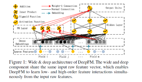
DeepFM包含两部分,左边的FM部分和右边的DNN部分。这两部分共享相同的输入。对于给定的特征ii, wiwi用于表示一阶特征的重要性,特征ii的隐向量(latent vector)ViVi用户表示和其他特征的相互影响。在FM部分,ViVi用于表征二阶特征,同时在神经网络部分用于构建高阶特征。对于当前模型,所有的参数共同参与训练。DeepFM的预测结果可以写为
y=sigmoid(yFM+yDNN)y=sigmoid(yFM+yDNN)
y∈(0,1)y∈(0,1)是预测的CTR,yFMyFM是FM部分得到的结果,yDNN是DNN部分的结果yDNN是DNN部分的结果
对于FM部分, 其计算公式和模型如下。详细可以看第一节,这里不在赘述
yFM=w0+∑ni=1wixi+∑ni=1∑nj=i+1<Vi,Vj>xixjyFM=w0+∑i=1nwixi+∑i=1n∑j=i+1n<Vi,Vj>xixj

对于神经网络DNN部分,其模型如下所示:
深度部分是一个前馈神经网络,可以学习高阶的特征组合。需要注意的是原始的输入的数据是很多个字段的高维稀疏数据。因此引入一个embedding layer将输入向量压缩到低维稠密向量。
embedding layer的结构如下图所示,
embedding layer有两个有趣的特性:
- 输入数据的每个字段的特征经过embedding之后,都为kk维(lantent vector的维度),所以embedding后的特征维度是 字段数×k字段数×k
- 在FM里得到的隐变量VV现在作为了嵌入层网络的权重,FM模型作为整个模型的一部分与其他深度学习模型一起参与整体的学习, 实现端到端的训练。
将embedding layer表征如下:
a(0)=[e1,e2,...,em]a(0)=[e1,e2,...,em]
eiei是第ii个字段的embedding,mm是字段的个数。a(0)a(0)是输入神经网络的向量,然后通过如下方式前向传播:
al+1=σ(W(l)a(l)+b(l))al+1=σ(W(l)a(l)+b(l))
需要指出的是,FM部分与深度部分共享相同的embedding带来了两个好处:
- 从原始数据中同时学习到了低维与高维特征
- 不再需要特征工程。而Wide&Deep Model需要
关于DNN网络结构的设计,文中给出的结果是,对于hidden layer, 使用三层200-200-200的结构设计。使用relu函数作为激活函数,增加了dropout。当然,关于超参数的调试,这个还要具体情况具体分析,只有手动取调试才知道哪些参数组合更好
代码实现
同样的,这里只给出FFM类的代码,详细代码见github,https://github.com/Johnson0722/CTR_Prediction/tree/master
class DeepFM(object):
    """
    Deep FM with FTRL optimization
    """
    def __init__(self, config):
        """
        :param config: configuration of hyperparameters
        type of dict
        """
        # number of latent factors
        self.k = config['k']
        self.lr = config['lr']
        self.batch_size = config['batch_size']
        self.reg_l1 = config['reg_l1']
        self.reg_l2 = config['reg_l2']
        # num of features
        self.p = feature_length
        # num of fields
        self.field_cnt = field_cnt

    def add_placeholders(self):
        self.X = tf.placeholder('float32', [None, self.p])
        self.y = tf.placeholder('int64', [None,])
        # index of none-zero features
        self.feature_inds = tf.placeholder('int64', [None,field_cnt])
        self.keep_prob = tf.placeholder('float32')

    def inference(self):
        """
        forward propagation
        :return: labels for each sample
        """
        v = tf.Variable(tf.truncated_normal(shape=[self.p, self.k], mean=0, stddev=0.01),dtype='float32')

        # Factorization Machine
        with tf.variable_scope('FM'):
            b = tf.get_variable('bias', shape=[2],
                                initializer=tf.zeros_initializer())
            w1 = tf.get_variable('w1', shape=[self.p, 2],
                                 initializer=tf.truncated_normal_initializer(mean=0,stddev=1e-2))
            # shape of [None, 2]
            self.linear_terms = tf.add(tf.matmul(self.X, w1), b)

            # shape of [None, 1]
            self.interaction_terms = tf.multiply(0.5,
                                                 tf.reduce_mean(
                                                     tf.subtract(
                                                         tf.pow(tf.matmul(self.X, v), 2),
                                                         tf.matmul(tf.pow(self.X, 2), tf.pow(v, 2))),
                                                     1, keep_dims=True))
            # shape of [None, 2]
            self.y_fm = tf.add(self.linear_terms, self.interaction_terms)

        # three-hidden-layer neural network, network shape of (200-200-200)
        with tf.variable_scope('DNN',reuse=False):
            # embedding layer
            y_embedding_input = tf.reshape(tf.gather(v, self.feature_inds), [-1, self.field_cnt*self.k])
            # first hidden layer
            w1 = tf.get_variable('w1_dnn', shape=[self.field_cnt*self.k, 200],
                                 initializer=tf.truncated_normal_initializer(mean=0,stddev=1e-2))
            b1 = tf.get_variable('b1_dnn', shape=[200],
                                 initializer=tf.constant_initializer(0.001))
            y_hidden_l1 = tf.nn.relu(tf.matmul(y_embedding_input, w1) + b1)
            # second hidden layer
            w2 = tf.get_variable('w2', shape=[200, 200],
                                 initializer=tf.truncated_normal_initializer(mean=0,stddev=1e-2))
            b2 = tf.get_variable('b2', shape=[200],
                                 initializer=tf.constant_initializer(0.001))
            y_hidden_l2 = tf.nn.relu(tf.matmul(y_hidden_l1, w2) + b2)
            # third hidden layer
            w3 = tf.get_variable('w1', shape=[200, 200],
                                 initializer=tf.truncated_normal_initializer(mean=0,stddev=1e-2))
            b3 = tf.get_variable('b1', shape=[200],
                                 initializer=tf.constant_initializer(0.001))
            y_hidden_l3 = tf.nn.relu(tf.matmul(y_hidden_l2, w3) + b3)
            # output layer
            w_out = tf.get_variable('w_out', shape=[200, 2],
                                 initializer=tf.truncated_normal_initializer(mean=0,stddev=1e-2))
            b_out = tf.get_variable('b_out', shape=[2],
                                 initializer=tf.constant_initializer(0.001))
            self.y_dnn = tf.nn.relu(tf.matmul(y_hidden_l3, w_out) + b_out)
        # add FM output and DNN output
        self.y_out = tf.add(self.y_fm, self.y_dnn)
        self.y_out_prob = tf.nn.softmax(self.y_out)

    def add_loss(self):
        cross_entropy = tf.nn.sparse_softmax_cross_entropy_with_logits(labels=self.y, logits=self.y_out)
        mean_loss = tf.reduce_mean(cross_entropy)
        self.loss = mean_loss
        tf.summary.scalar('loss', self.loss)

    def add_accuracy(self):
        # accuracy
        self.correct_prediction = tf.equal(tf.cast(tf.argmax(model.y_out,1), tf.int64), model.y)
        self.accuracy = tf.reduce_mean(tf.cast(self.correct_prediction, tf.float32))
        # add summary to accuracy# CTR预估算法之FM, FFM, DeepFM及实践# CTR预估算法之FM, FFM, DeepFM及实践c

   tf.summary.scalar('accuracy', self.accuracy)

    def train(self):
        # Applies exponential decay to learning rate
        self.global_step = tf.Variable(0, trainable=False)
        # define optimizer
        optimizer = tf.train.FtrlOptimizer(self.lr, l1_regularization_strength=self.reg_l1,
                                           l2_regularization_strength=self.reg_l2)
        extra_update_ops = tf.get_collection(tf.GraphKeys.UPDATE_OPS)
        with tf.control_dependencies(extra_update_ops):
            self.train_op = optimizer.minimize(self.loss, global_step=self.global_step)

    def build_graph(self):
        """build graph for model"""
        self.add_placeholders()
        self.inference()
        self.add_loss()
        self.add_accuracy()
        self.train()
参考文献
1.https://en.wikipedia.org/wiki/Click-through_rate
2.http://blog.csdn.net/g11d111/article/details/77430095
3.https://tech.meituan.com/deep-understanding-of-ffm-principles-and-practices.html
4.http://www.csie.ntu.edu.tw/~r01922136/slides/ffm.pdf
5.http://baijiahao.baidu.com/s?id=1579855367208283187&wfr=spider&for=pc
--------------------- 本文来自 Johnson0722 的CSDN 博客 ,全文地址请点击:https://blog.csdn.net/john_xyz/article/details/78933253?utm_source=copy


 3165
3165


 被折叠的 条评论
为什么被折叠?
被折叠的 条评论
为什么被折叠?
 到【灌水乐园】发言


