机器学习中的数学——距离定义（二十五）：布雷格曼散度（Bregman Divergence）

分类目录：《机器学习中的数学》总目录
相关文章：
· 距离定义：基础知识
· 距离定义（一）：欧几里得距离（Euclidean Distance）
· 距离定义（二）：曼哈顿距离（Manhattan Distance）
· 距离定义（三）：闵可夫斯基距离（Minkowski Distance）
· 距离定义（四）：切比雪夫距离（Chebyshev Distance）
· 距离定义（五）：标准化的欧几里得距离（Standardized Euclidean Distance）
· 距离定义（六）：马氏距离（Mahalanobis Distance）
· 距离定义（七）：兰氏距离（Lance and Williams Distance）/堪培拉距离（Canberra Distance）
· 距离定义（八）：余弦距离（Cosine Distance）
· 距离定义（九）：测地距离（Geodesic Distance）
· 距离定义（十）： 布雷柯蒂斯距离（Bray Curtis Distance）
· 距离定义（十一）：汉明距离（Hamming Distance）
· 距离定义（十二）：编辑距离（Edit Distance，Levenshtein Distance）
· 距离定义（十三）：杰卡德距离（Jaccard Distance）和杰卡德相似系数（Jaccard Similarity Coefficient）
· 距离定义（十四）：Ochiia系数（Ochiia Coefficient）
· 距离定义（十五）：Dice系数（Dice Coefficient）
· 距离定义（十六）：豪斯多夫距离（Hausdorff Distance）
· 距离定义（十七）：皮尔逊相关系数（Pearson Correlation）
· 距离定义（十八）：卡方距离（Chi-square Measure）
· 距离定义（十九）：交叉熵（Cross Entropy）
· 距离定义（二十）：相对熵（Relative Entropy）/KL散度（Kullback-Leibler Divergence）
· 距离定义（二十一）：JS散度（Jensen–Shannon Divergence）
· 距离定义（二十二）：海林格距离（Hellinger Distance）
· 距离定义（二十三）：α-散度（α-Divergence）
· 距离定义（二十四）：F-散度（F-Divergence）
· 距离定义（二十五）：布雷格曼散度（Bregman Divergence）
· 距离定义（二十六）：Wasserstein距离（Wasserstei Distance）/EM距离（Earth-Mover Distance）
· 距离定义（二十七）：巴氏距离（Bhattacharyya Distance）
· 距离定义（二十八）：最大均值差异（Maximum Mean Discrepancy, MMD）
· 距离定义（二十九）：点间互信息（Pointwise Mutual Information, PMI）

---

F-散度已经可以表达我们提到的所有散度，目前为止它是最通用的散度形式。但很多文章也会出现另一种叫做Bregman的散度，它和F-散度不太一样，是另一大类散度。

我们以欧几里得距离举例，即$n$维空间中的欧几里得距离：
$$d(x,y)=\sqrt{\sum _{i=1}^n(x_i-y_i{)}^2}$$

我们将其平方：
$$d^2(x,y)=\sum _{i=1}^n(x_i-y_i{)}^2$$

如果我们定义内积$<x,y>={\sum }_{i-1}^n{x}_i{y}_i$和欧式模$||x||=\sqrt{<x,x>}$，则上式可以写为如下形式：
$$d^2(x,y)=\sum _{i=1}^n(x_i-y_i{)}^2=<x-y,x-y>=||x|{|}^2-(||y|{|}^2+<2y,x-y>)$$

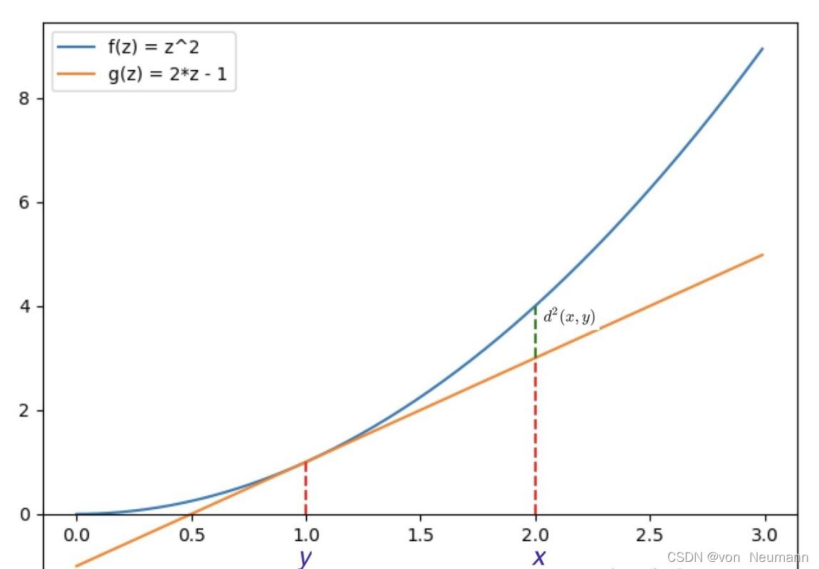
注意到，$2y$是$y^2$的导数，因此上式的后一项$(||y|{|}^2+<2y,x-y>$是函数$f(z)=||z|{|}^2$在$y$点的切线在$x$处的取值。所以均方欧几里得距离的几何描述便是欧式模函数在点$x$和其在$y$点切线在点估计的差。如下图绿线所示：

那么一个很自然的想法就是把这个定义拓展，即对任意$R^n$的函数$f(x)$，我们都可以定义：
$$d(x,y)=f(x)-(f(y)+<\nabla f(y),x-y>)$$

若$f(x)$是凸函数，则可以保证$d(x,y)\ge 0$，上式也是Bregman散度（Bregman Divergence）的定义。

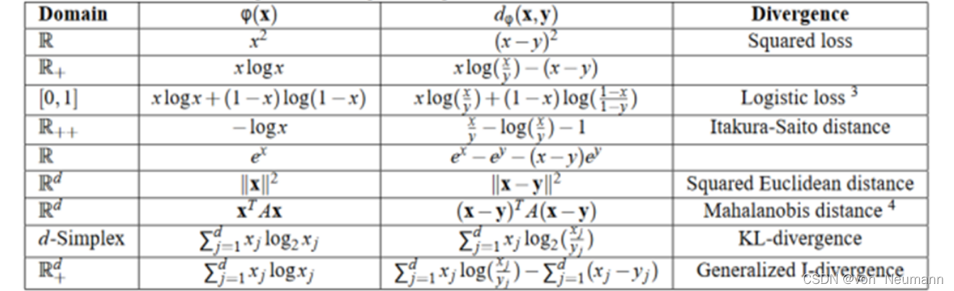
和F-散度类似，Bregman散度也是一大类散度的通用表达形式，具体的，根据$f(x)$取不同的函数，它可以表示不同的散度，其中KL散度也是它的一个特例：