C4.5决策树+代码实践

--------------------------------文章修改于4月1日———————————————————

之前的文章排版有点混乱，概念不清，代码没仔细整理过。发现许多人使用这个代码，特此修改这篇blog，希望改进后能叙述地更清晰明朗。

 

决策树是一种非线性分类器，每次根据某个规则，选择一个特征，并以某个特征的某个值为阈值，把训练样本递归的分为若干子树。以同样的规则递归划分，最后得到一棵可用于决策分类的树形分类器。

实例 

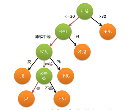
转载一个简单的决策树实例如下

通俗来说，决策树分类的思想类似于找对象。现想象一个女孩的母亲要给这个女孩介绍男朋友，于是有了下面的对话：

     女儿：多大年纪了？

     母亲：26。

     女儿：长的帅不帅？

     母亲：挺帅的。

     女儿：收入高不？

     母亲：不算很高，中等情况。

     女儿：是公务员不？

     母亲：是，在税务局上班呢。

     女儿：那好，我去见见。

 

     这个女孩的决策过程就是典型的分类树决策。相当于通过年龄、长相、收入和是否公务员对将男人分为两个类别：见和不见。假设这个女孩对男人的要求是：30岁以下、长相中等以上并且是高收入者或中等以上收入的公务员，那么这个可以用下图表示女孩的决策逻辑。

 

非线性分类器

如果特征向量是二维的，我们还能用一个二维空间上的图来说明。

下面是一个二维决策树。

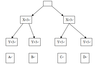
上述决策树的构造可以在二维平面上如下表示：

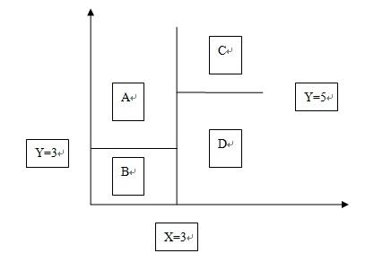
可见，决策树是非线性的分类器。

划分规则

ID3与C4.5都是以信息熵为划分，目的是寻找一个最佳的划分方法。不过ID与C4.5都是贪心的方式，也就是每次选择当前最优解，并不一定能达到整体最优解。

信息熵：

D表示某个样本的分布，那么这时候的样本不确定可以用如下的公式衡量：

 

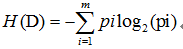
其中p表示概率分布。

信息熵表示一个分布的不确定度，在这里也就是类别的不确定度。如果都为同一类，那么不确定度为0。

如果我们把决策树的构造当做一个信息不确定度不断减小，直至能确定为某个类的过程，那么每次划分，只要使得当前信息熵最小化就行。

现在我们假设将训练元组D按属性A进行划分，那么已知划分事件A，D的不确定度为：

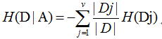
Dj表示划分后的第j个子树样本的分布，绝对值表示个数，H(Dj)表示如此划分后第j个子树的信息熵。

而信息增益即为两者的差值：

 

我们画个图来说明：

 

所谓的互信息I（A;D），就是已知A后，我们得到的D的信息。互信息越大，我们的划分越纯粹。

那么ID3的方法就是每次选择划分事件A与分布D互信息最大的划分方法。

ID3局限性

经证明，ID有如下局限性：

*只能处理特征值是离散值的情况

（因为ID3默认以离散值来划分）

*使用信息增益作为节点的分裂标准，实际上并不合理，会倾向于选择取值较多的属性。

（极端情况下，N个属性N个样本标签，得到N个子树，每个子树信息熵为0，总信息熵为0。具体的数学推导未知）

*并没有剪枝操作，容易发生过拟合的现象

*无法处理缺失值

（由于其只处理离散值的情况，不能解决不存在的值）

 

C4.5

C4.5加入了信息增益率。因为经证明，划分事件A，划分的子树越多，其熵H（A）越大。如下图：

 

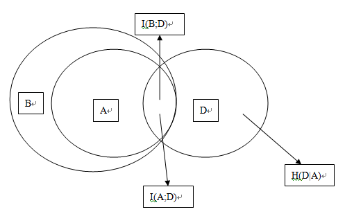
两个划分方法，A，B。B的划分数大于A，一般情况下有H（B）>H(A)，上图中以面积大小表示。

（*因为划分为3个子树，可以看成先划分为两个，在把其中一个划分为两个。所以，多次划分的信息熵一般是大于少次的。极端情况下，N个属性N个样本标签，得到N个子树，每个子树信息熵为0，总信息熵为0，这样的划分是没有意义的）

他们与D的交集， I（B,D）>I（A,D）。根据ID3，我们会偏向选择B，也就是偏向于多划分的。于是我们引入如下的增益率。

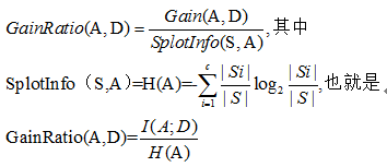
即把I(A;D)做一个归一化处理，在上图中看来就是把交集的面积除以本身面积得到一个比值而不是绝对数值，从而避免ID3倾向更多划分的情况。

其中的分母正比于子树的个数、

 

代码实践

决策树的生成是一个NP难题，一般如上两种算法，采用贪心的策略，递归生成树，但并不能保证全局最优解。

 

递归建树时，有如下的结束条件：

1.集合中只剩一类特征，结束递归，子树的类别为此类。

2.集合中个数小于设置的某个参数，如5%的原始数据大小，结束递归，子树类别为较多的一类。

其中条件2是防止过拟合的条件。

 

然后是关于代码：

1.网上的代码即有离散方法，又有连续方法。一般来说，我们要把属性值处理为离散的方法，这里改代码是偷了个懒，直接离散化为两类。

2.其记录方法的错误，导致程序出错，整理如下：

*对于离散的变量，（程序中可设置值类别大于10的为离散），如[1,3,6,8]，用来建树的话，如果测试输入未出现的5，出错。

*连续变量。如果出现[6,6,6,6,7,7,7],计算记录在7的地方划分，就会分为[6,6,6,6,7,7,7]和空集[]。

 

针对程序的这些问题，做如下修改：

1.删去离散的方法，直接全部当做连续变量处理。（主要是不知道如何处理离散值的miss value 问题）

2.划分改为记录位置，而不是记录值。

3.一般的决策树还有剪枝的各个策略来防止过拟合，暂时没有加入这些功能。

 

改完后得到的matlab代码如下：

function D = C4_5(train_features, train_targets, inc_node,test_features)


[Ni, M]		= size(train_features); %输入向量为NI*M的矩阵，其中M表示训练样本个数，Ni为特征维数维数
inc_node    = inc_node*M/100; 

disp('Building tree') 
tree        = make_tree(train_features, train_targets, inc_node); 
 
%Make the decision region according to the tree %根据产生的数产生决策域
disp('Building decision surface using the tree') 
[n,m]=size(test_features);
targets		= use_tree(test_features, 1:m, tree, unique(train_targets)); %target里包含了对应的测试样本分类所得的类别数
 
D   		= targets; 
%END 
 
function targets = use_tree(features, indices, tree,  Uc) %target里包含了对应的测试样本分类所得的类别
 

targets = zeros(1, size(features,2)); %1*M的向量
 
if (tree.dim == 0) 
   %Reached the end of the tree 
   targets(indices) = tree.child; 
   return %child里面包含了类别信息，indeces包含了测试样本中当前测试的样本索引
end 
         

dim = tree.dim; %当前节点的特征参数
dims= 1:size(features,1); %dims为1-特征维数的向量
 
   %Discrete feature 
   in				= indices(find(features(dim, indices) <= tree.split_loc)); %in为左子树在原矩阵的index

   targets		= targets + use_tree(features(dims, :), in, tree.child_1, Uc); 
   in				= indices(find(features(dim, indices) >  tree.split_loc)); 

   targets		= targets + use_tree(features(dims, :), in, tree.child_2, Uc); 
return 
      
 
function tree = make_tree(features, targets, inc_node) 

[Ni, L]    					= size(features); 
Uc         					= unique(targets); %UC表示类别数
tree.dim						= 0; %数的维度为0
%tree.child(1:maxNbin)	= zeros(1,maxNbin); 
 
if isempty(features), %如果特征为空，退出
   return 
end 

%When to stop: If the dimension is one or the number of examples is small 
if ((inc_node > L) | (L == 1) | (length(Uc) == 1)), %剩余训练集只剩一个，或太小，小于inc_node，或只剩一类，退出
   H					= hist(targets, length(Uc)); %返回类别数的直方图
   [m, largest] 	= max(H); %更大的一类，m为大的值，即个数，largest为位置，即类别的位置
   tree.child	 	= Uc(largest); %直接返回其中更大的一类作为其类别
   return
end 
 
%Compute the node's I 
%计算现有的信息量
for i = 1:length(Uc), 
    Pnode(i) = length(find(targets == Uc(i))) / L; 
end 
Inode = -sum(Pnode.*log(Pnode)/log(2)); 
 
%For each dimension, compute the gain ratio impurity 
%This is done separately for discrete and continuous features 
delta_Ib    = zeros(1, Ni); 
S=[];
for i = 1:Ni, 
   data	= features(i,:); 
   temp=unique(data); 
      P	= zeros(length(Uc), 2); 
       
      %Sort the features 
      [sorted_data, indices] = sort(data); 
      sorted_targets = targets(indices); 
       %结果为排序后的特征和类别
      %Calculate the information for each possible split 
      I	= zeros(1, L-1); 
      
      for j = 1:L-1, 
         for k =1:length(Uc), 
            P(k,1) = length(find(sorted_targets(1:j) 		== Uc(k))); 
            P(k,2) = length(find(sorted_targets(j+1:end) == Uc(k))); 
         end 
         Ps		= sum(P)/L; %两个子树的权重 
         temp1=[P(:,1)]; 
         temp2=[P(:,2)]; 
         fo=[Info(temp1),Info(temp2)];
         %info	= sum(-P.*log(eps+P)/log(2)); %两个子树的I
         I(j)	= Inode - sum(fo.*Ps);    
      end 
      [delta_Ib(i), s] = max(I); 
      S=[S,s];
   
end
 
%Find the dimension minimizing delta_Ib  
%找到最大的划分方法
[m, dim] = max(delta_Ib); 

dims		= 1:Ni; 
tree.dim = dim; 

%Split along the 'dim' dimension 
%分裂树 
   %Continuous feature 
   [sorted_data, indices] = sort(features(dim,:)); 
   %tree.split_loc		= split_loc(dim); 
   %disp(tree.split_loc);
   S(dim)
   indices1=indices(1:S(dim))
   indices2=indices(S(dim)+1:end)
   tree.split_loc=sorted_data(S(dim))
   tree.child_1		= make_tree(features(dims, indices1), targets(indices1), inc_node); 
   tree.child_2		= make_tree(features(dims, indices2), targets(indices2), inc_node); 
%D = C4_5_new(train_features, train_targets, inc_node);

还有就是自己写的计算集合熵的函数：

function I=Info(A)
L=sum(A);
A=A/L;
I=-sum(A.*log(A+eps)/log(2));

以上是根据自己的理解和自己的解决方式改写的代码，有不完善的地方以后发现后再慢慢改进。

 

最后，回答几个关于代码的问题：

1.      train_features,为训练集； train_targets,为训练集标签；inc_node为防止过拟合参数，表示样本数小于一定阈值结束递归，可设置为5-10；test_features为测试集。

2.      取消离散变量，上面说了，是因为我不知道如何处理Miss value的问题，至于影响，应该就是连贪心也算不上了吧，应该是一个理论上还过得去的处理方法。

3.      图怎么画？介绍几个画图软件：http://www.cnblogs.com/damonlan/archive/2012/03/29/2410301.html 

决策树扩展篇：http://blog.csdn.net/ice110956/article/details/29175215