


Part 1
We've spent the last couple of months on QuantStart backtesting various trading strategies utilising Python and pandas. The vectorised nature of pandas ensures that certain operations on large datasets are extremely rapid. However the forms of vectorised backtester that we have studied to date suffer from some drawbacks in the way that trade execution is simulated. In this series of articles we are going to discuss a more realistic approach to historical strategy simulation by constructing an event-driven backtesting environment using Python.
Event-Driven Software
Before we delve into development of such a backtester we need to understand the concept of event-driven systems. Video games provide a natural use case for event-driven software and provide a straightforward example to explore. A video game has multiple components that interact with each other in a real-time setting at high framerates. This is handled by running the entire set of calculations within an "infinite" loop known as the event-loop or game-loop.
At each tick of the game-loop a function is called to receive the latest event, which will have been generated by some corresponding prior action within the game. Depending upon the nature of the event, which could include a key-press or a mouse click, some subsequent action is taken, which will either terminate the loop or generate some additional events. The process will then continue. Here is some example pseudo-code:
while True:  # Run the loop forever
    new_event = get_new_event()   # Get the latest event

    # Based on the event type, perform an action
    if new_event.type == "LEFT_MOUSE_CLICK":
        open_menu()
    elif new_event.type == "ESCAPE_KEY_PRESS":
        quit_game()
    elif new_event.type == "UP_KEY_PRESS":
        move_player_north()
    # ... and many more events

    redraw_screen()   # Update the screen to provide animation
    tick(50)   # Wait 50 milliseconds
The code is continually checking for new events and then performing actions based on these events. In particular it allows the illusion of real-time response handling because the code is continually being looped and events checked for. As will become clear this is precisely what we need in order to carry out high frequency trading simulation.
Why An Event-Driven Backtester?
Event-driven systems provide many advantages over a vectorised approach:
- Code Reuse - An event-driven backtester, by design, can be used for both historical backtesting and live trading with minimal switch-out of components. This is not true of vectorised backtesters where all data must be available at once to carry out statistical analysis.
- Lookahead Bias - With an event-driven backtester there is no lookahead bias as market data receipt is treated as an "event" that must be acted upon. Thus it is possible to "drip feed" an event-driven backtester with market data, replicating how an order management and portfolio system would behave.
- Realism - Event-driven backtesters allow significant customisation over how orders are executed and transaction costs are incurred. It is straightforward to handle basic market and limit orders, as well as market-on-open (MOO) and market-on-close (MOC), since a custom exchange handler can be constructed.
Although event-driven systems come with many benefits they suffer from two major disadvantages over simpler vectorised systems. Firstly they are significantly more complex to implement and test. There are more "moving parts" leading to a greater chance of introducing bugs. To mitigate this proper software testing methodology such as test-driven development can be employed.
Secondly they are slower to execute compared to a vectorised system. Optimal vectorised operations are unable to be utilised when carrying out mathematical calculations. We will discuss ways to overcome these limitations in later articles.
Event-Driven Backtester Overview
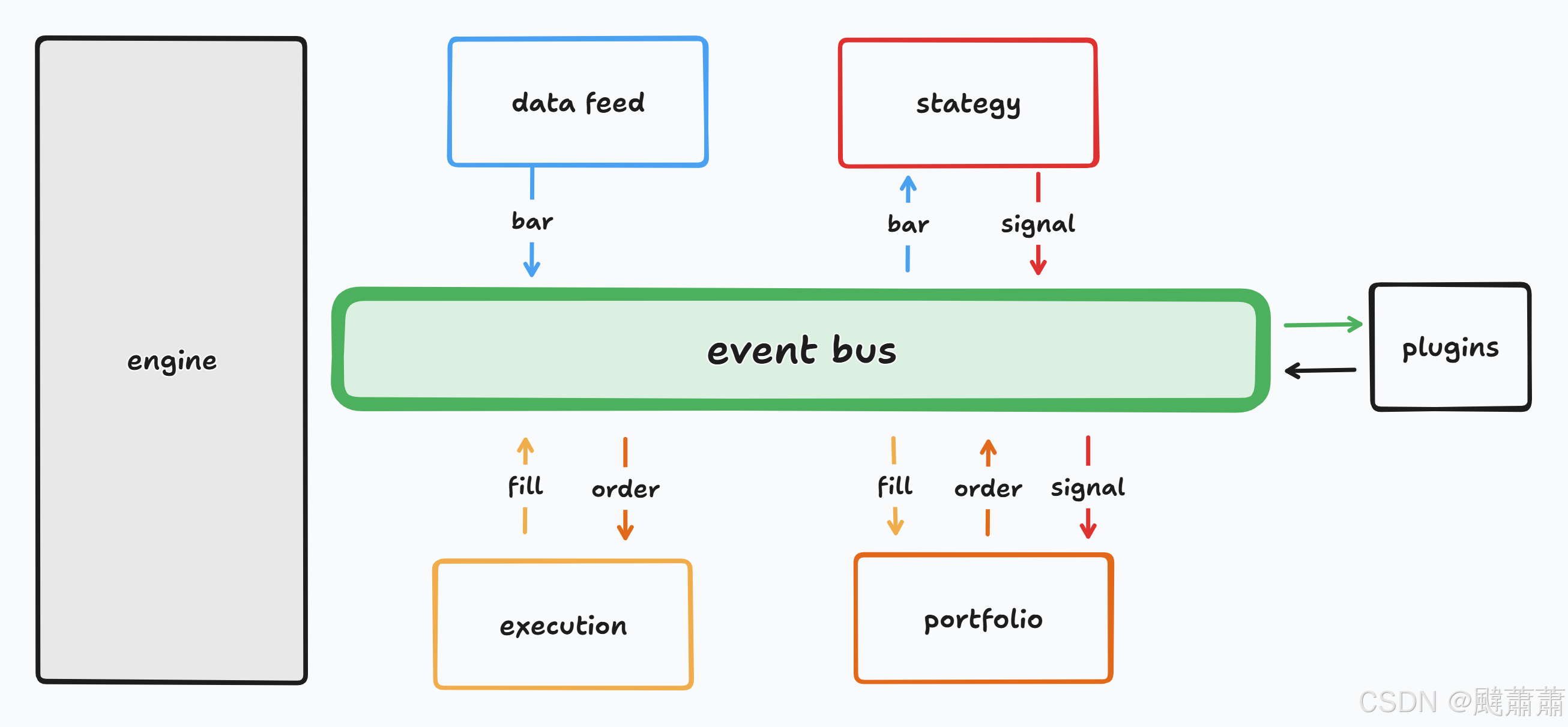
To apply an event-driven approach to a backtesting system it is necessary to define our components (or objects) that will handle specific tasks:
- Event - The
Eventis the fundamental class unit of the event-driven system. It contains a type (such as "MARKET", "SIGNAL", "ORDER" or "FILL") that determines how it will be handled within the event-loop. - Event Queue - The Event Queue is an in-memory Python Queue object that stores all of the Event sub-class objects that are generated by the rest of the software.
- DataHandler - The
DataHandleris an abstract base class (ABC) that presents an interface for handling both historical or live market data. This provides significant flexibility as the Strategy and Portfolio modules can thus be reused between both approaches. The DataHandler generates a newMarketEventupon every heartbeat of the system (see below). - Strategy - The
Strategyis also an ABC that presents an interface for taking market data and generating corresponding SignalEvents, which are ultimately utilised by the Portfolio object. A SignalEvent contains a ticker symbol, a direction (LONG or SHORT) and a timestamp. - Portfolio - This is an ABC which handles the order management associated with current and subsequent positions for a strategy. It also carries out risk management across the portfolio, including sector exposure and position sizing. In a more sophisticated implementation this could be delegated to a RiskManagement class. The
Portfoliotakes SignalEvents from the Queue and generates OrderEvents that get added to the Queue. - ExecutionHandler - The
ExecutionHandlersimulates a connection to a brokerage. The job of the handler is to take OrderEvents from the Queue and execute them, either via a simulated approach or an actual connection to a liver brokerage. Once orders are executed the handler creates FillEvents, which describe what was actually transacted, including fees, commission and slippage (if modelled). - The Loop - All of these components are wrapped in an event-loop that correctly handles all Event types, routing them to the appropriate component.
This is quite a basic model of a trading engine. There is significant scope for expansion, particularly in regard to how the Portfolio is used. In addition differing transaction cost models might also be abstracted into their own class hierarchy. At this stage it introduces needless complexity within this series of articles so we will not currently discuss it further. In later tutorials we will likely expand the system to include additional realism.
Here is a snippet of Python code that demonstrates how the backtester works in practice. There are two loops occuring in the code. The outer loop is used to give the backtester a heartbeat. For live trading this is the frequency at which new market data is polled. For backtesting strategies this is not strictly necessary since the backtester uses the market data provided in drip-feed form (see the bars.update_bars() line).
The inner loop actually handles the Events from the events Queue object. Specific events are delegated to the respective component and subsequently new events are added to the queue. When the events Queue is empty, the heartbeat loop continues:
# Declare the components with respective parameters
bars = DataHandler(..)
strategy = Strategy(..)
port = Portfolio(..)
broker = ExecutionHandler(..)

while True:
    # Update the bars (specific backtest code, as opposed to live trading)
    if bars.continue_backtest == True:
        bars.update_bars()
    else:
        break

    # Handle the events
    while True:
        try:
            event = events.get(False)
        except Queue.Empty:
            break
        else:
            if event is not None:
                if event.type == 'MARKET':
                    strategy.calculate_signals(event)
                    port.update_timeindex(event)

                elif event.type == 'SIGNAL':
                    port.update_signal(event)

                elif event.type == 'ORDER':
                    broker.execute_order(event)

                elif event.type == 'FILL':
                    port.update_fill(event)

    # 10-Minute heartbeat
    time.sleep(10*60)
This is the basic outline of a how an event-driven backtester is designed. In the next article we will discuss the Event class hierarchy.
Part 2
In the last article we described the concept of an event-driven backtester. The remainder of this series of articles will concentrate on each of the separate class hierarchies that make up the overall system. In this article we will consider Events and how they can be used to communicate information between objects.
As discussed in the previous article the trading system utilises two while loops - an outer and an inner. The inner while loop handles capture of events from an in-memory queue, which are then routed to the appropriate component for subsequent action. In this infrastucture there are four types of events:
- MarketEvent - This is triggered when the outer while loop begins a new "heartbeat". It occurs when the
DataHandlerobject receives a new update of market data for any symbols which are currently being tracked. It is used to trigger theStrategyobject generating new trading signals. The event object simply contains an identification that it is a market event, with no other structure. - SignalEvent - The
Strategyobject utilises market data to create newSignalEvents. TheSignalEventcontains a ticker symbol, a timestamp for when it was generated and a direction (long or short). TheSignalEvents are utilised by thePortfolioobject as advice for how to trade. - OrderEvent - When a
Portfolioobject receivesSignalEvents it assesses them in the wider context of the portfolio, in terms of risk and position sizing. This ultimately leads toOrderEvents that will be sent to anExecutionHandler. - FillEvent - When an
ExecutionHandlerreceives anOrderEventit must transact the order. Once an order has been transacted it generates aFillEvent, which describes the cost of purchase or sale as well as the transaction costs, such as fees or slippage.
The parent class is called Event. It is a base class and does not provide any functionality or specific interface. In later implementations the Event objects will likely develop greater complexity and thus we are future-proofing the design of such systems by creating a class hierarchy.
# event.py

class Event(object):
    """
    Event is base class providing an interface for all subsequent
    (inherited) events, that will trigger further events in the
    trading infrastructure.
    """
    pass
The MarketEvent inherits from Event and provides little more than a self-identification that it is a 'MARKET' type event.
# event.py

class MarketEvent(Event):
    """
    Handles the event of receiving a new market update with
    corresponding bars.
    """

    def __init__(self):
        """
        Initialises the MarketEvent.
        """
        self.type = 'MARKET'
A SignalEvent requires a ticker symbol, a timestamp for generation and a direction in order to advise a Portfolio object.
# event.py

class SignalEvent(Event):
    """
    Handles the event of sending a Signal from a Strategy object.
    This is received by a Portfolio object and acted upon.
    """

    def __init__(self, symbol, datetime, signal_type):
        """
        Initialises the SignalEvent.

        Parameters:
        symbol - The ticker symbol, e.g. 'GOOG'.
        datetime - The timestamp at which the signal was generated.
        signal_type - 'LONG' or 'SHORT'.
        """

        self.type = 'SIGNAL'
        self.symbol = symbol
        self.datetime = datetime
        self.signal_type = signal_type
The OrderEvent is slightly more complex than a SignalEvent since it contains a quantity field in addition to the aforementioned properties of SignalEvent. The quantity is determined by the Portfolio constraints. In addition the OrderEvent has a print_order() method, used to output the information to the console if necessary.
# event.py

class OrderEvent(Event):
    """
    Handles the event of sending an Order to an execution system.
    The order contains a symbol (e.g. GOOG), a type (market or limit),
    quantity and a direction.
    """

    def __init__(self, symbol, order_type, quantity, direction):
        """
        Initialises the order type, setting whether it is
        a Market order ('MKT') or Limit order ('LMT'), has
        a quantity (integral) and its direction ('BUY' or
        'SELL').

        Parameters:
        symbol - The instrument to trade.
        order_type - 'MKT' or 'LMT' for Market or Limit.
        quantity - Non-negative integer for quantity.
        direction - 'BUY' or 'SELL' for long or short.
        """

        self.type = 'ORDER'
        self.symbol = symbol
        self.order_type = order_type
        self.quantity = quantity
        self.direction = direction

    def print_order(self):
        """
        Outputs the values within the Order.
        """
        print "Order: Symbol=%s, Type=%s, Quantity=%s, Direction=%s" % \
            (self.symbol, self.order_type, self.quantity, self.direction)
The FillEvent is the Event with the greatest complexity. It contains a timestamp for when an order was filled, the symbol of the order and the exchange it was executed on, the quantity of shares transacted, the actual price of the purchase and the commission incurred.
The commission is calculated using the Interactive Brokers commissions. For US API orders this commission is 1.30 USD minimum per order, with a flat rate of either 0.013 USD or 0.08 USD per share depending upon whether the trade size is below or above 500 units of stock.
# event.py

class FillEvent(Event):
    """
    Encapsulates the notion of a Filled Order, as returned
    from a brokerage. Stores the quantity of an instrument
    actually filled and at what price. In addition, stores
    the commission of the trade from the brokerage.
    """

    def __init__(self, timeindex, symbol, exchange, quantity,
                 direction, fill_cost, commission=None):
        """
        Initialises the FillEvent object. Sets the symbol, exchange,
        quantity, direction, cost of fill and an optional
        commission.

        If commission is not provided, the Fill object will
        calculate it based on the trade size and Interactive
        Brokers fees.

        Parameters:
        timeindex - The bar-resolution when the order was filled.
        symbol - The instrument which was filled.
        exchange - The exchange where the order was filled.
        quantity - The filled quantity.
        direction - The direction of fill ('BUY' or 'SELL')
        fill_cost - The holdings value in dollars.
        commission - An optional commission sent from IB.
        """

        self.type = 'FILL'
        self.timeindex = timeindex
        self.symbol = symbol
        self.exchange = exchange
        self.quantity = quantity
        self.direction = direction
        self.fill_cost = fill_cost

        # Calculate commission
        if commission is None:
            self.commission = self.calculate_ib_commission()
        else:
            self.commission = commission

    def calculate_ib_commission(self):
        """
        Calculates the fees of trading based on an Interactive
        Brokers fee structure for API, in USD.

        This does not include exchange or ECN fees.

        Based on "US API Directed Orders":
        https://www.interactivebrokers.com/en/index.php?f=commission&p=stocks2
        """
        full_cost = 1.3
        if self.quantity <= 500:
            full_cost = max(1.3, 0.013 * self.quantity)
        else: # Greater than 500
            full_cost = max(1.3, 0.008 * self.quantity)
        full_cost = min(full_cost, 0.5 / 100.0 * self.quantity * self.fill_cost)
        return full_cost
In the next article of the series we are going to consider how to develop a market DataHandler class hierarchy that allows both historic backtesting and live trading, via the same class interface.
Part 3
In the previous two articles of the series we discussed what an event-driven backtesting system is and the class hierarchy for the Event object. In this article we are going to consider how market data is utilised, both in a historical backtesting context and for live trade execution.
One of our goals with an event-driven trading system is to minimise duplication of code between the backtesting element and the live execution element. Ideally it would be optimal to utilise the same signal generation methodology and portfolio management components for both historical testing and live trading. In order for this to work the Strategy object which generates the Signals, and the Portfolio object which provides Orders based on them, must utilise an identical interface to a market feed for both historic and live running.
This motivates the concept of a class hierarchy based on a DataHandler object, which gives all subclasses an interface for providing market data to the remaining components within the system. In this way any subclass data handler can be "swapped out", without affecting strategy or portfolio calculation.
Specific example subclasses could include HistoricCSVDataHandler, QuandlDataHandler, SecuritiesMasterDataHandler, InteractiveBrokersMarketFeedDataHandler etc. In this tutorial we are only going to consider the creation of a historic CSV data handler, which will load intraday CSV data for equities in an Open-Low-High-Close-Volume-OpenInterest set of bars. This can then be used to "drip feed" on a bar-by-bar basis the data into the Strategy and Portfolio classes on every heartbeat of the system, thus avoiding lookahead bias.
The first task is to import the necessary libraries. Specifically we are going to import pandas and the abstract base class tools. Since the DataHandler generates MarketEvents we also need to import event.py as described in the previous tutorial:
# data.py

import datetime
import os, os.path
import pandas as pd

from abc import ABCMeta, abstractmethod

from event import MarketEvent
The DataHandler is an abstract base class (ABC), which means that it is impossible to instantiate an instance directly. Only subclasses may be instantiated. The rationale for this is that the ABC provides an interface that all subsequent DataHandler subclasses must adhere to thereby ensuring compatibility with other classes that communicate with them.
We make use of the __metaclass__ property to let Python know that this is an ABC. In addition we use the @abstractmethod decorator to let Python know that the method will be overridden in subclasses (this is identical to a pure virtual method in C++).
The two methods of interest are get_latest_bars and update_bars. The former returns the last $N$ bars from the current heartbeat timestamp, which is useful for rolling calculations needed in Strategy classes. The latter method provides a "drip feed" mechanism for placing bar information on a new data structure that strictly prohibits lookahead bias. Notice that exceptions will be raised if an attempted instantiation of the class occurs:
# data.py

class DataHandler(object):
    """
    DataHandler is an abstract base class providing an interface for
    all subsequent (inherited) data handlers (both live and historic).

    The goal of a (derived) DataHandler object is to output a generated
    set of bars (OLHCVI) for each symbol requested.

    This will replicate how a live strategy would function as current
    market data would be sent "down the pipe". Thus a historic and live
    system will be treated identically by the rest of the backtesting suite.
    """

    __metaclass__ = ABCMeta

    @abstractmethod
    def get_latest_bars(self, symbol, N=1):
        """
        Returns the last N bars from the latest_symbol list,
        or fewer if less bars are available.
        """
        raise NotImplementedError("Should implement get_latest_bars()")

    @abstractmethod
    def update_bars(self):
        """
        Pushes the latest bar to the latest symbol structure
        for all symbols in the symbol list.
        """
        raise NotImplementedError("Should implement update_bars()")
With the DataHandler ABC specified the next step is to create a handler for historic CSV files. In particular the HistoricCSVDataHandler will take multiple CSV files, one for each symbol, and convert these into a dictionary of pandas DataFrames.
The data handler requires a few parameters, namely an Event Queue on which to push MarketEvent information to, the absolute path of the CSV files and a list of symbols. Here is the initialisation of the class:
# data.py

class HistoricCSVDataHandler(DataHandler):
    """
    HistoricCSVDataHandler is designed to read CSV files for
    each requested symbol from disk and provide an interface
    to obtain the "latest" bar in a manner identical to a live
    trading interface.
    """

    def __init__(self, events, csv_dir, symbol_list):
        """
        Initialises the historic data handler by requesting
        the location of the CSV files and a list of symbols.

        It will be assumed that all files are of the form
        'symbol.csv', where symbol is a string in the list.

        Parameters:
        events - The Event Queue.
        csv_dir - Absolute directory path to the CSV files.
        symbol_list - A list of symbol strings.
        """
        self.events = events
        self.csv_dir = csv_dir
        self.symbol_list = symbol_list

        self.symbol_data = {}
        self.latest_symbol_data = {}
        self.continue_backtest = True

        self._open_convert_csv_files()
It will implicitly try to open the files with the format of "SYMBOL.csv" where symbol is the ticker symbol. The format of the files matches that provided by Yahoo, but is easily modified to handle additional data formats. The opening of the files is handled by the _open_convert_csv_files method below.
One of the benefits of using pandas as a datastore internally within the HistoricCSVDataHandler is that the indexes of all symbols being tracked can be merged together. This allows missing data points to be padded forward, backward or interpolated within these gaps such that tickers can be compared on a bar-to-bar basis. This is necessary for mean-reverting strategies, for instance. Notice the use of the union and reindex methods when combining the indexes for all symbols:
# data.py

    def _open_convert_csv_files(self):
        """
        Opens the CSV files from the data directory, converting
        them into pandas DataFrames within a symbol dictionary.

        For this handler it will be assumed that the data is
        taken from Yahoo. Thus its format will be respected.
        """
        comb_index = None
        for s in self.symbol_list:
            # Load the CSV file with no header information, indexed on date
            self.symbol_data[s] = pd.read_csv(
                os.path.join(self.csv_dir, '%s.csv' % s),
                header=0, index_col=0, parse_dates=True,
                names=[
                    'datetime', 'open', 'high',
                    'low', 'close', 'adj_close', 'volume'
                ]
            )
            self.symbol_data[s].sort_index(inplace=True)

            # Combine the index to pad forward values
            if comb_index is None:
                comb_index = self.symbol_data[s].index
            else:
                comb_index.union(self.symbol_data[s].index)

            # Set the latest symbol_data to None
            self.latest_symbol_data[s] = []

        for s in self.symbol_list:
            self.symbol_data[s] = self.symbol_data[s].reindex(
                index=comb_index, method='pad'
            )
            self.symbol_data[s]["returns"] = self.symbol_data[s]["adj_close"].pct_change().dropna()
            self.symbol_data[s] = self.symbol_data[s].iterrows()

        # Reindex the dataframes
        for s in self.symbol_list:
            self.symbol_data[s] = self.symbol_data[s].reindex(index=comb_index, method='pad').iterrows()
The _get_new_bar method creates a generator to provide a formatted version of the bar data. This means that subsequent calls to the method will yield a new bar until the end of the symbol data is reached:
# data.py

    def _get_new_bar(self, symbol):
        """
        Returns the latest bar from the data feed as a tuple of
        (sybmbol, datetime, open, low, high, close, volume).
        """
        for b in self.symbol_data[symbol]:
            yield tuple([symbol, datetime.datetime.strptime(b[0], '%Y-%m-%d %H:%M:%S'),
                        b[1][0], b[1][1], b[1][2], b[1][3], b[1][4]])
The first abstract method from DataHandler to be implemented is get_latest_bars. This method simply provides a list of the last $N$ bars from the latest_symbol_data structure. Setting $N=1$ allows the retrieval of the current bar (wrapped in a list):
# data.py

    def get_latest_bars(self, symbol, N=1):
        """
        Returns the last N bars from the latest_symbol list,
        or N-k if less available.
        """
        try:
            bars_list = self.latest_symbol_data[symbol]
        except KeyError:
            print "That symbol is not available in the historical data set."
        else:
            return bars_list[-N:]
The final method, update_bars, is the second abstract method from DataHandler. It simply generates a MarketEvent that gets added to the queue as it appends the latest bars to the latest_symbol_data:
# data.py

    def update_bars(self):
        """
        Pushes the latest bar to the latest_symbol_data structure
        for all symbols in the symbol list.
        """
        for s in self.symbol_list:
            try:
                bar = self._get_new_bar(s).next()
            except StopIteration:
                self.continue_backtest = False
            else:
                if bar is not None:
                    self.latest_symbol_data[s].append(bar)
        self.events.put(MarketEvent())
Thus we have a DataHandler-derived object, which is used by the remaining components to keep track of market data. The Strategy, Portfolio and ExecutionHandler objects all require the current market data thus it makes sense to centralise it to avoid duplication of storage.
In the next article we will consider the Strategy class hierarchy and describe how a strategy can be designed to handle multiple symbols, thus generating multiple SignalEvents for the Portfolio object.
Part 4
The discussion of the event-driven backtesting implementation has previously considered the event-loop, the event class hierarchy and the data handling component. In this article a Strategy class hierarchy will be outlined. Strategy objects take market data as input and produce trading signal events as output.
A Strategy object encapsulates all calculations on market data that generate advisory signals to a Portfolio object. At this stage in the event-driven backtester development there is no concept of an indicator or filter, such as those found in technical trading. These are also good candidates for creating a class hierarchy but are beyond the scope of this article.
The strategy hierarchy is relatively simple as it consists of an abstract base class with a single pure virtual method for generating SignalEvent objects. In order to create the Strategy hierarchy it is necessary to import NumPy, pandas, the Queue object, abstract base class tools and the SignalEvent:
# strategy.py

import datetime
import numpy as np
import pandas as pd
import Queue

from abc import ABCMeta, abstractmethod

from event import SignalEvent
The Strategy abstract base class simply defines a pure virtual calculate_signals method. In derived classes this is used to handle the generation of SignalEvent objects based on market data updates:
# strategy.py

class Strategy(object):
    """
    Strategy is an abstract base class providing an interface for
    all subsequent (inherited) strategy handling objects.

    The goal of a (derived) Strategy object is to generate Signal
    objects for particular symbols based on the inputs of Bars
    (OLHCVI) generated by a DataHandler object.

    This is designed to work both with historic and live data as
    the Strategy object is agnostic to the data source,
    since it obtains the bar tuples from a queue object.
    """

    __metaclass__ = ABCMeta

    @abstractmethod
    def calculate_signals(self):
        """
        Provides the mechanisms to calculate the list of signals.
        """
        raise NotImplementedError("Should implement calculate_signals()")
The definition of the Strategy ABC is straightforward. Our first example of subclassing the Strategy object makes use of a buy and hold strategy to create the BuyAndHoldStrategy class. This simply goes long in a particular security on a certain date and keeps it within the portfolio. Thus only one signal per security is ever generated.
The constructor (__init__) requires the bars market data handler and the events event queue object:
# strategy.py

class BuyAndHoldStrategy(Strategy):
    """
    This is an extremely simple strategy that goes LONG all of the
    symbols as soon as a bar is received. It will never exit a position.

    It is primarily used as a testing mechanism for the Strategy class
    as well as a benchmark upon which to compare other strategies.
    """

    def __init__(self, bars, events):
        """
        Initialises the buy and hold strategy.

        Parameters:
        bars - The DataHandler object that provides bar information
        events - The Event Queue object.
        """
        self.bars = bars
        self.symbol_list = self.bars.symbol_list
        self.events = events

        # Once buy & hold signal is given, these are set to True
        self.bought = self._calculate_initial_bought()
On initialisation of the BuyAndHoldStrategy the bought dictionary member has a set of keys for each symbol that are all set to False. Once the asset has been "longed" then this is set to True. Essentially this allows the Strategy to know whether it is "in the market" or not:
# strategy.py

    def _calculate_initial_bought(self):
        """
        Adds keys to the bought dictionary for all symbols
        and sets them to False.
        """
        bought = {}
        for s in self.symbol_list:
            bought[s] = False
        return bought
The calculate_signals pure virtual method is implemented concretely in this class. The method loops over all symbols in the symbol list and retrieves the latest bar from the bars data handler. It then checks whether that symbol has been "bought" (i.e. whether we're in the market for this symbol or not) and if not creates a single SignalEvent object. This is then placed on the events queue and the bought dictionary is correctly updated to True for this particular symbol key:
# strategy.py

    def calculate_signals(self, event):
        """
        For "Buy and Hold" we generate a single signal per symbol
        and then no additional signals. This means we are
        constantly long the market from the date of strategy
        initialisation.

        Parameters
        event - A MarketEvent object.
        """
        if event.type == 'MARKET':
            for s in self.symbol_list:
                bars = self.bars.get_latest_bars(s, N=1)
                if bars is not None and bars != []:
                    if self.bought[s] == False:
                        # (Symbol, Datetime, Type = LONG, SHORT or EXIT)
                        signal = SignalEvent(bars[0][0], bars[0][1], 'LONG')
                        self.events.put(signal)
                        self.bought[s] = True
This is clearly a simple strategy but it is sufficient to demonstrate the nature of an event-driven strategy hierarchy. In subsequent articles we will consider more sophisticated strategies such as a pairs trade. In the next article we will consider how to create a Portfolio hierarchy that keeps track of our positions with a profit and loss ("PnL").
Part 5
In the previous article on event-driven backtesting we considered how to construct a Strategy class hierarchy. Strategies, as defined here, are used to generate signals, which are used by a portfolio object in order to make decisions on whether to send orders. As before it is natural to create a Portfolio abstract base class (ABC) that all subsequent subclasses inherit from.
This article describes a NaivePortfolio object that keeps track of the positions within a portfolio and generates orders of a fixed quantity of stock based on signals. Later portfolio objects will include more sophisticated risk management tools and will be the subject of later articles.
Position Tracking and Order Management
The portfolio order management system is possibly the most complex component of an event-driven backtester. Its role is to keep track of all current market positions as well as the market value of the positions (known as the "holdings"). This is simply an estimate of the liquidation value of the position and is derived in part from the data handling facility of the backtester.
In addition to the positions and holdings management the portfolio must also be aware of risk factors and position sizing techniques in order to optimise orders that are sent to a brokerage or other form of market access.
Continuing in the vein of the Event class hierarchy a Portfolio object must be able to handle SignalEvent objects, generate OrderEvent objects and interpret FillEvent objects to update positions. Thus it is no surprise that the Portfolio objects are often the largest component of event-driven systems, in terms of lines of code (LOC).
Implementation
We create a new file portfolio.py and import the necessary libraries. These are the same as most of the other abstract base class implementations. We need to import the floor function from the math library in order to generate integer-valued order sizes. We also need the FillEvent and OrderEvent objects since the Portfolio handles both.
# portfolio.py

import datetime
import numpy as np
import pandas as pd
import Queue

from abc import ABCMeta, abstractmethod
from math import floor

from event import FillEvent, OrderEvent
As before we create an ABC for Portfolio and have two pure virtual methods update_signal and update_fill. The former handles new trading signals being grabbed from the events queue and the latter handles fills received from an execution handler object.
# portfolio.py

class Portfolio(object):
    """
    The Portfolio class handles the positions and market
    value of all instruments at a resolution of a "bar",
    i.e. secondly, minutely, 5-min, 30-min, 60 min or EOD.
    """

    __metaclass__ = ABCMeta

    @abstractmethod
    def update_signal(self, event):
        """
        Acts on a SignalEvent to generate new orders
        based on the portfolio logic.
        """
        raise NotImplementedError("Should implement update_signal()")

    @abstractmethod
    def update_fill(self, event):
        """
        Updates the portfolio current positions and holdings
        from a FillEvent.
        """
        raise NotImplementedError("Should implement update_fill()")
The principal subject of this article is the NaivePortfolio class. It is designed to handle position sizing and current holdings, but will carry out trading orders in a "dumb" manner by simply sending them directly to the brokerage with a predetermined fixed quantity size, irrespective of cash held. These are all unrealistic assumptions, but they help to outline how a portfolio order management system (OMS) functions in an event-driven fashion.
The NaivePortfolio requires an initial capital value, which I have set to the default of 100,000 USD. It also requires a starting date-time.
The portfolio contains the all_positions and current_positions members. The former stores a list of all previous positions recorded at the timestamp of a market data event. A position is simply the quantity of the asset. Negative positions mean the asset has been shorted. The latter member stores a dictionary containing the current positions for the last market bar update.
In addition to the positions members the portfolio stores holdings, which describe the current market value of the positions held. "Current market value" in this instance means the closing price obtained from the current market bar, which is clearly an approximation, but is reasonable enough for the time being. all_holdings stores the historical list of all symbol holdings, while current_holdings stores the most up to date dictionary of all symbol holdings values.
# portfolio.py

class NaivePortfolio(Portfolio):
    """
    The NaivePortfolio object is designed to send orders to
    a brokerage object with a constant quantity size blindly,
    i.e. without any risk management or position sizing. It is
    used to test simpler strategies such as BuyAndHoldStrategy.
    """

    def __init__(self, bars, events, start_date, initial_capital=100000.0):
        """
        Initialises the portfolio with bars and an event queue.
        Also includes a starting datetime index and initial capital
        (USD unless otherwise stated).

        Parameters:
        bars - The DataHandler object with current market data.
        events - The Event Queue object.
        start_date - The start date (bar) of the portfolio.
        initial_capital - The starting capital in USD.
        """
        self.bars = bars
        self.events = events
        self.symbol_list = self.bars.symbol_list
        self.start_date = start_date
        self.initial_capital = initial_capital

        self.all_positions = self.construct_all_positions()
        self.current_positions = dict( (k,v) for k, v in [(s, 0) for s in self.symbol_list] )

        self.all_holdings = self.construct_all_holdings()
        self.current_holdings = self.construct_current_holdings()
The following method, construct_all_positions, simply creates a dictionary for each symbol, sets the value to zero for each and then adds a datetime key, finally adding it to a list. It uses a dictionary comprehension, which is similar in spirit to a list comprehension:
# portfolio.py

    def construct_all_positions(self):
        """
        Constructs the positions list using the start_date
        to determine when the time index will begin.
        """
        d = dict( (k,v) for k, v in [(s, 0) for s in self.symbol_list] )
        d['datetime'] = self.start_date
        return [d]
The construct_all_holdings method is similar to the above but adds extra keys for cash, commission and total, which respectively represent the spare cash in the account after any purchases, the cumulative commission accrued and the total account equity including cash and any open positions. Short positions are treated as negative. The starting cash and total account equity are both set to the initial capital:
# portfolio.py

    def construct_all_holdings(self):
        """
        Constructs the holdings list using the start_date
        to determine when the time index will begin.
        """
        d = dict( (k,v) for k, v in [(s, 0.0) for s in self.symbol_list] )
        d['datetime'] = self.start_date
        d['cash'] = self.initial_capital
        d['commission'] = 0.0
        d['total'] = self.initial_capital
        return [d]
The following method, construct_current_holdings is almost identical to the method above except that it doesn't wrap the dictionary in a list:
# portfolio.py

    def construct_current_holdings(self):
        """
        This constructs the dictionary which will hold the instantaneous
        value of the portfolio across all symbols.
        """
        d = dict( (k,v) for k, v in [(s, 0.0) for s in self.symbol_list] )
        d['cash'] = self.initial_capital
        d['commission'] = 0.0
        d['total'] = self.initial_capital
        return d
On every "heartbeat", that is every time new market data is requested from the DataHandler object, the portfolio must update the current market value of all the positions held. In a live trading scenario this information can be downloaded and parsed directly from the brokerage, but for a backtesting implementation it is necessary to calculate these values manually.
Unfortunately there is no such as thing as the "current market value" due to bid/ask spreads and liquidity issues. Thus it is necessary to estimate it by multiplying the quantity of the asset held by a "price". The approach I have taken here is to use the closing price of the last bar received. For an intraday strategy this is relatively realistic. For a daily strategy this is less realistic as the opening price can differ substantially from the closing price.
The method update_timeindex handles the new holdings tracking. It firstly obtains the latest prices from the market data handler and creates a new dictionary of symbols to represent the current positions, by setting the "new" positions equal to the "current" positions. These are only changed when a FillEvent is obtained, which is handled later on in the portfolio. The method then appends this set of current positions to the all_positions list. Next, the holdings are updated in a similar manner, with the exception that the market value is recalculated by multiplying the current positions count with the closing price of the latest bar (self.current_positions[s] * bars[s][0][5]). Finally the new holdings are appended to all_holdings:
# portfolio.py

    def update_timeindex(self, event):
        """
        Adds a new record to the positions matrix for the current
        market data bar. This reflects the PREVIOUS bar, i.e. all
        current market data at this stage is known (OLHCVI).

        Makes use of a MarketEvent from the events queue.
        """
        bars = {}
        for sym in self.symbol_list:
            bars[sym] = self.bars.get_latest_bars(sym, N=1)

        # Update positions
        dp = dict( (k,v) for k, v in [(s, 0) for s in self.symbol_list] )
        dp['datetime'] = bars[self.symbol_list[0]][0][1]

        for s in self.symbol_list:
            dp[s] = self.current_positions[s]

        # Append the current positions
        self.all_positions.append(dp)

        # Update holdings
        dh = dict( (k,v) for k, v in [(s, 0) for s in self.symbol_list] )
        dh['datetime'] = bars[self.symbol_list[0]][0][1]
        dh['cash'] = self.current_holdings['cash']
        dh['commission'] = self.current_holdings['commission']
        dh['total'] = self.current_holdings['cash']

        for s in self.symbol_list:
            # Approximation to the real value
            market_value = self.current_positions[s] * bars[s][0][5]
            dh[s] = market_value
            dh['total'] += market_value

        # Append the current holdings
        self.all_holdings.append(dh)
The method update_positions_from_fill determines whether a FillEvent is a Buy or a Sell and then updates the current_positions dictionary accordingly by adding/subtracting the correct quantity of shares:
# portfolio.py

    def update_positions_from_fill(self, fill):
        """
        Takes a FilltEvent object and updates the position matrix
        to reflect the new position.

        Parameters:
        fill - The FillEvent object to update the positions with.
        """
        # Check whether the fill is a buy or sell
        fill_dir = 0
        if fill.direction == 'BUY':
            fill_dir = 1
        if fill.direction == 'SELL':
            fill_dir = -1

        # Update positions list with new quantities
        self.current_positions[fill.symbol] += fill_dir*fill.quantity
The corresponding update_holdings_from_fill is similar to the above method but updates the holdings values instead. In order to simulate the cost of a fill, the following method does not use the cost associated from the FillEvent. Why is this? Simply put, in a backtesting environment the fill cost is actually unknown and thus is must be estimated. Thus the fill cost is set to the the "current market price" (the closing price of the last bar). The holdings for a particular symbol are then set to be equal to the fill cost multiplied by the transacted quantity.
Once the fill cost is known the current holdings, cash and total values can all be updated. The cumulative commission is also updated:
# portfolio.py

    def update_holdings_from_fill(self, fill):
        """
        Takes a FillEvent object and updates the holdings matrix
        to reflect the holdings value.

        Parameters:
        fill - The FillEvent object to update the holdings with.
        """
        # Check whether the fill is a buy or sell
        fill_dir = 0
        if fill.direction == 'BUY':
            fill_dir = 1
        if fill.direction == 'SELL':
            fill_dir = -1

        # Update holdings list with new quantities
        fill_cost = self.bars.get_latest_bars(fill.symbol)[0][5]  # Close price
        cost = fill_dir * fill_cost * fill.quantity
        self.current_holdings[fill.symbol] += cost
        self.current_holdings['commission'] += fill.commission
        self.current_holdings['cash'] -= (cost + fill.commission)
        self.current_holdings['total'] -= (cost + fill.commission)
The pure virtual update_fill method from the Portfolio ABC is implemented here. It simply executes the two preceding methods, update_positions_from_fill and update_holdings_from_fill, which have already been discussed above:
# portfolio.py

    def update_fill(self, event):
        """
        Updates the portfolio current positions and holdings
        from a FillEvent.
        """
        if event.type == 'FILL':
            self.update_positions_from_fill(event)
            self.update_holdings_from_fill(event)
While the Portfolio object must handle FillEvents, it must also take care of generating OrderEvents upon the receipt of one or more SignalEvents. The generate_naive_order method simply takes a signal to long or short an asset and then sends an order to do so for 100 shares of such an asset. Clearly 100 is an arbitrary value. In a realistic implementation this value will be determined by a risk management or position sizing overlay. However, this is a NaivePortfolio and so it "naively" sends all orders directly from the signals, without a risk system.
The method handles longing, shorting and exiting of a position, based on the current quantity and particular symbol. Corresponding OrderEvent objects are then generated:
# portfolio.py

    def generate_naive_order(self, signal):
        """
        Simply transacts an OrderEvent object as a constant quantity
        sizing of the signal object, without risk management or
        position sizing considerations.

        Parameters:
        signal - The SignalEvent signal information.
        """
        order = None

        symbol = signal.symbol
        direction = signal.signal_type
        strength = signal.strength

        mkt_quantity = floor(100 * strength)
        cur_quantity = self.current_positions[symbol]
        order_type = 'MKT'

        if direction == 'LONG' and cur_quantity == 0:
            order = OrderEvent(symbol, order_type, mkt_quantity, 'BUY')
        if direction == 'SHORT' and cur_quantity == 0:
            order = OrderEvent(symbol, order_type, mkt_quantity, 'SELL')

        if direction == 'EXIT' and cur_quantity > 0:
            order = OrderEvent(symbol, order_type, abs(cur_quantity), 'SELL')
        if direction == 'EXIT' and cur_quantity < 0:
            order = OrderEvent(symbol, order_type, abs(cur_quantity), 'BUY')
        return order
The update_signal method simply calls the above method and adds the generated order to the events queue:
# portfolio.py

    def update_signal(self, event):
        """
        Acts on a SignalEvent to generate new orders
        based on the portfolio logic.
        """
        if event.type == 'SIGNAL':
            order_event = self.generate_naive_order(event)
            self.events.put(order_event)
The final method in the NaivePortfolio is the generation of an equity curve. This simply creates a returns stream, useful for performance calculations and then normalises the equity curve to be percentage based. Thus the account initial size is equal to 1.0:
# portfolio.py

    def create_equity_curve_dataframe(self):
        """
        Creates a pandas DataFrame from the all_holdings
        list of dictionaries.
        """
        curve = pd.DataFrame(self.all_holdings)
        curve.set_index('datetime', inplace=True)
        curve['returns'] = curve['total'].pct_change()
        curve['equity_curve'] = (1.0+curve['returns']).cumprod()
        self.equity_curve = curve
The Portfolio object is the most complex aspect of the entire event-driven backtest system. The implementation here, while intricate, is relatively elementary in its handling of positions. Later versions will consider risk management and position sizing, which will lead to a much more realistic idea of strategy performance.
In the next article we will consider the final piece of the event-driven backtester, namely an ExecutionHandler object, which is used to take OrderEvent objects and create FillEvent objects from them.
Part 6
This article continues the discussion of event-driven backtesters in Python. In the previous article we considered a portfolio class hierarchy that handled current positions, generated trading orders and kept track of profit and loss (PnL).
In this article we will study the execution of these orders, by creating a class hierarchy that will represent a simulated order handling mechanism and ultimately tie into a brokerage or other means of market connectivity.
The ExecutionHandler described here is exceedingly simple, since it fills all orders at the current market price. This is highly unrealistic, but serves as a good baseline for improvement.
As with the previous abstract base class hierarchies, we must import the necessary properties and decorators from the abc library. In addition we need to import the FillEvent and OrderEvent:
# execution.py

import datetime
import Queue

from abc import ABCMeta, abstractmethod

from event import FillEvent, OrderEvent
The ExecutionHandler is similar to previous abstract base classes and simply has one pure virtual method, execute_order:
# execution.py

class ExecutionHandler(object):
    """
    The ExecutionHandler abstract class handles the interaction
    between a set of order objects generated by a Portfolio and
    the ultimate set of Fill objects that actually occur in the
    market.

    The handlers can be used to subclass simulated brokerages
    or live brokerages, with identical interfaces. This allows
    strategies to be backtested in a very similar manner to the
    live trading engine.
    """

    __metaclass__ = ABCMeta

    @abstractmethod
    def execute_order(self, event):
        """
        Takes an Order event and executes it, producing
        a Fill event that gets placed onto the Events queue.

        Parameters:
        event - Contains an Event object with order information.
        """
        raise NotImplementedError("Should implement execute_order()")
In order to backtest strategies we need to simulate how a trade will be transacted. The simplest possible implementation is assumes all orders are filled at the current market price for all quantities. This is clearly extremely unrealistic and a big part of improving backtest realism will come from designing more sophisticated models of slippage and market impact.
Note that the FillEvent is given a value of None for the fill_cost (see the penultimate line in execute_order) as the we have already taken care of the cost of fill in the NaivePortfolio object described in the previous article. In a more realistic implementation we would make use of the "current" market data value to obtain a realistic fill cost.
I have simply utilised ARCA as the exchange although for backtesting purposes this is purely a placeholder. In a live execution environment this venue dependence would be far more important:
# execution.py

class SimulatedExecutionHandler(ExecutionHandler):
    """
    The simulated execution handler simply converts all order
    objects into their equivalent fill objects automatically
    without latency, slippage or fill-ratio issues.

    This allows a straightforward "first go" test of any strategy,
    before implementation with a more sophisticated execution
    handler.
    """

    def __init__(self, events):
        """
        Initialises the handler, setting the event queues
        up internally.

        Parameters:
        events - The Queue of Event objects.
        """
        self.events = events

    def execute_order(self, event):
        """
        Simply converts Order objects into Fill objects naively,
        i.e. without any latency, slippage or fill ratio problems.

        Parameters:
        event - Contains an Event object with order information.
        """
        if event.type == 'ORDER':
            fill_event = FillEvent(datetime.datetime.utcnow(), event.symbol,
                                   'ARCA', event.quantity, event.direction, None)
            self.events.put(fill_event)
This concludes the class hierarchies necessary to produce an event-driven backtester. In the next article we will discuss how to calculate a set of performance metrics for the backtested strategy.
Part 7
In the last article on the Event-Driven Backtester series we considered a basic ExecutionHandler hierarchy. In this article we are going to discuss how to assess the performance of a strategy post-backtest using the previously constructed equity curve DataFrame in the Portfolio object.
Performance Metrics
We've already considered the Sharpe Ratio in a previous article. In that article I outline that the (annualised) Sharpe ratio is calculated via:
\begin{eqnarray*}
S_A = \sqrt{N} \frac{\mathbb{E}(R_a - R_b)}{\sqrt{\text{Var} (R_a - R_b)}}
\end{eqnarray*}
Where $R_a$ is the returns stream of the equity curve and $R_b$ is a benchmark, such as an appropriate interest rate or equity index.
The maximum drawdown and drawdown duration are two additional measures that investors often uses to assess the risk in a portfolio. The former quantities the highest peak-to-trough decline in an equity curve performance, while the latter is defined as the number of trading periods over which it occurs.
In this article we will implement the Sharpe ratio, maximum drawdown and drawdown duration as measures of portfolio performance for use in the Python-based Event-Driven Backtesting suite.
Python Implementation
The first task is to create a new file performance.py, which stores the functions to calculate the Sharpe ratio and drawdown information. As with most of our calculation-heavy classes we need to import NumPy and pandas:
# performance.py

import numpy as np
import pandas as pd
Note that the Sharpe ratio is a measure of risk to reward (in fact it is one of many!). It has a single parameter, that of the number of periods to adjust for when scaling up to the annualised value.
Usually this value is set to 252, which is the number of trading days in the US per year. However, if your strategy trades within the hour you need to adjust the Sharpe to correctly annualise it. Thus you need to set periods to $252*6.5 = 1638$, which is the number of US trading hours within a year. If you trade on a minutely basis, then this factor must be set to $252*6.5*60=98280$.
The create_sharpe_ratio function operates on a pandas Series object called returns and simply calculates the ratio of the mean of the period percentage returns and the period percentage return standard deviations scaled by the periods factor:
# performance.py

def create_sharpe_ratio(returns, periods=252):
    """
    Create the Sharpe ratio for the strategy, based on a
    benchmark of zero (i.e. no risk-free rate information).

    Parameters:
    returns - A pandas Series representing period percentage returns.
    periods - Daily (252), Hourly (252*6.5), Minutely(252*6.5*60) etc.
    """
    return np.sqrt(periods) * (np.mean(returns)) / np.std(returns)
While the Sharpe ratio characterises how much risk (as defined by asset path standard deviation) is being taken per unit of return, the "drawdown" is defined as the largest peak-to-trough drop along an equity curve.
The create_drawdowns function below actually provides both the maximum drawdown and the maximum drawdown duration. The former is the aforementioned largest peak-to-trough drop, while the latter is defined as the number of periods over which this drop occurs.
There is some subtlety required in the interpretation of the drawdown duration as it counts trading periods and thus is not directly translateable into a temporal unit such as "days".
The function starts by creating two pandas Series objects representing the drawdown and duration at each trading "bar". Then the current high water mark (HWM) is established by determining if the equity curve exceeds all previous peaks.
The drawdown is then simply the difference between the current HWM and the equity curve. If this value is negative then the duration is increased for every bar that this occurs until the next HWM is reached. The function then simply returns the maximum of each of the two Series:
# performance.py

def create_drawdowns(equity_curve):
    """
    Calculate the largest peak-to-trough drawdown of the PnL curve
    as well as the duration of the drawdown. Requires that the
    pnl_returns is a pandas Series.

    Parameters:
    pnl - A pandas Series representing period percentage returns.

    Returns:
    drawdown, duration - Highest peak-to-trough drawdown and duration.
    """

    # Calculate the cumulative returns curve
    # and set up the High Water Mark
    # Then create the drawdown and duration series
    hwm = [0]
    eq_idx = equity_curve.index
    drawdown = pd.Series(index = eq_idx, dtype=float)
    duration = pd.Series(index = eq_idx, dtype=float)

    # Loop over the index range
    for t in range(1, len(eq_idx)):
        cur_hwm = max(hwm[t-1], equity_curve[t])
        hwm.append(cur_hwm)
        drawdown[t]= hwm[t] - equity_curve[t]
        duration[t]= 0 if drawdown[t] == 0 else duration[t-1] + 1
    return drawdown.max(), duration.max()
In order to make use of these performance measures we need a means of calculating them after a backtest has been carried out, i.e. when a suitable equity curve is available!
We also need to associate the calculation with a particular object hierarchy. Given that the performance measures are calculated on a portfolio basis, it makes sense to attach the performance calculations to a method on the Portfolio class hierarchy that we discussed in this article.
The first task is to open up portfolio.py as discussed in the previous article and import the performance functions:
# portfolio.py

..  # Other imports

from performance import create_sharpe_ratio, create_drawdowns
Since Portfolio is an abstract base class we want to attach a method to one of its derived classes, which in this case will be NaivePortfolio. Hence we will create a method called output_summary_stats that will act on the portfolio equity curve to generate the Sharpe and drawdown information.
The method is straightforward. It simply utilises the two performance measures and applies them directly to the equity curve pandas DataFrame, outputting the statistics as a list of tuples in a format-friendly manner:
# portfolio.py

..
..

class NaivePortfolio(object):

    ..
    ..

    def output_summary_stats(self):
        """
        Creates a list of summary statistics for the portfolio such
        as Sharpe Ratio and drawdown information.
        """
        total_return = self.equity_curve['equity_curve'][-1]
        returns = self.equity_curve['returns']
        pnl = self.equity_curve['equity_curve']

        sharpe_ratio = create_sharpe_ratio(returns)
        max_dd, dd_duration = create_drawdowns(pnl)

        stats = [("Total Return", "%0.2f%%" % ((total_return - 1.0) * 100.0)),
                 ("Sharpe Ratio", "%0.2f" % sharpe_ratio),
                 ("Max Drawdown", "%0.2f%%" % (max_dd * 100.0)),
                 ("Drawdown Duration", "%d" % dd_duration)]
        return stats
Clearly this is a very simple performance analysis for a portfolio. It does not consider trade-level analysis or other measures of risk/reward. However it is straightforward to extend by adding more methods into performance.py and then incorporating them into output_summary_stats as required.
Part 8
It's been a while since we've considered the event-driven backtester, which we began discussing in this article. In Part VI I described how to code a stand-in ExecutionHandler model that worked for a historical backtesting situation. In this article we are going to code the corresponding Interactive Brokers API handler in order to move towards a live trading system.
I've previously discussed how to download Trader Workstation and create an Interactive Brokers demo account as well as how to create a basic interface to the IB API using IbPy. This article will wrap up the basic IbPy interface into the event-driven system, so that when it is paired with a live market feed, it will form the basis for an automated execution system.
The essential idea of the IBExecutionHandler class (see below) is to receive OrderEvent instances from the events queue and then to execute them directly against the Interactive Brokers order API using the IbPy library. The class will also handle the "Server Response" messages sent back via the API. At this stage, the only action taken will be to create corresponding FillEvent instances that will then be sent back to the events queue.
The class itself could feasibly become rather complex, with execution optimisation logic as well as sophisticated error handling. However, I have opted to keep it relatively simple so that you can see the main ideas and extend it in the direction that suits your particular trading style.
Python Implementation
As always, the first task is to create the Python file and import the necessary libraries. The file is called ib_execution.py and lives in the same directory as the other event-driven files.
We import the necessary date/time handling libraries, the IbPy objects and the specific Event objects that are handled by IBExecutionHandler:
# ib_execution.py

import datetime
import time

from ib.ext.Contract import Contract
from ib.ext.Order import Order
from ib.opt import ibConnection, message

from event import FillEvent, OrderEvent
from execution import ExecutionHandler
We now define the IBExecutionHandler class. The __init__ constructor firstly requires knowledge of the events queue. It also requires specification of order_routing, which I've defaulted to "SMART". If you have specific exchange requirements, you can specify them here. The default currency has also been set to US Dollars.
Within the method we create a fill_dict dictionary, needed later for usage in generating FillEvent instances. We also create a tws_conn connection object to store our connection information to the Interactive Brokers API. We also have to create an initial default order_id, which keeps track of all subsequent orders to avoid duplicates. Finally we register the message handlers (which we'll define in more detail below):
# ib_execution.py

class IBExecutionHandler(ExecutionHandler):
    """
    Handles order execution via the Interactive Brokers
    API, for use against accounts when trading live
    directly.
    """

    def __init__(self, events,
                 order_routing="SMART",
                 currency="USD"):
        """
        Initialises the IBExecutionHandler instance.
        """
        self.events = events
        self.order_routing = order_routing
        self.currency = currency
        self.fill_dict = {}

        self.tws_conn = self.create_tws_connection()
        self.order_id = self.create_initial_order_id()
        self.register_handlers()
The IB API utilises a message-based event system that allows our class to respond in particular ways to certain messages, in a similar manner to the event-driven backtester itself. I've not included any real error handling (for the purposes of brevity), beyond output to the terminal, via the _error_handler method.
The _reply_handler method, on the other hand, is used to determine if a FillEvent instance needs to be created. The method asks if an "openOrder" message has been received and checks whether an entry in our fill_dict for this particular orderId has already been set. If not then one is created.
If it sees an "orderStatus" message and that particular message states than an order has been filled, then it calls create_fill to create a FillEvent. It also outputs the message to the terminal for logging/debug purposes:
# ib_execution.py

    def _error_handler(self, msg):
        """
        Handles the capturing of error messages
        """
        # Currently no error handling.
        print "Server Error: %s" % msg

    def _reply_handler(self, msg):
        """
        Handles of server replies
        """
        # Handle open order orderId processing
        if msg.typeName == "openOrder" and \
            msg.orderId == self.order_id and \
            not self.fill_dict.has_key(msg.orderId):
            self.create_fill_dict_entry(msg)
        # Handle Fills
        if msg.typeName == "orderStatus" and \
            msg.status == "Filled" and \
            self.fill_dict[msg.orderId]["filled"] == False:
            self.create_fill(msg)
        print "Server Response: %s, %s\n" % (msg.typeName, msg)
The following method, create_tws_connection, creates a connection to the IB API using the IbPy ibConnection object. It uses a default port of 7496 and a default clientId of 10. Once the object is created, the connect method is called to perform the connection:
# ib_execution.py

    def create_tws_connection(self):
        """
        Connect to the Trader Workstation (TWS) running on the
        usual port of 7496, with a clientId of 10.
        The clientId is chosen by us and we will need
        separate IDs for both the execution connection and
        market data connection, if the latter is used elsewhere.
        """
        tws_conn = ibConnection()
        tws_conn.connect()
        return tws_conn
To keep track of separate orders (for the purposes of tracking fills) the following method create_initial_order_id is used. I've defaulted it to "1", but a more sophisticated approach would be th query IB for the latest available ID and use that. You can always reset the current API order ID via the Trader Workstation > Global Configuration > API Settings panel:
# ib_execution.py

    def create_initial_order_id(self):
        """
        Creates the initial order ID used for Interactive
        Brokers to keep track of submitted orders.
        """
        # There is scope for more logic here, but we
        # will use "1" as the default for now.
        return 1
The following method, register_handlers, simply registers the error and reply handler methods defined above with the TWS connection:
# ib_execution.py

    def register_handlers(self):
        """
        Register the error and server reply
        message handling functions.
        """
        # Assign the error handling function defined above
        # to the TWS connection
        self.tws_conn.register(self._error_handler, 'Error')

        # Assign all of the server reply messages to the
        # reply_handler function defined above
        self.tws_conn.registerAll(self._reply_handler)
As with the previous tutorial on using IbPy we need to create a Contract instance and then pair it with an Order instance, which will be sent to the IB API. The following method, create_contract, generates the first component of this pair. It expects a ticker symbol, a security type (e.g. stock or future), an exchange/primary exchange and a currency. It returns the Contract instance:
# ib_execution.py

    def create_contract(self, symbol, sec_type, exch, prim_exch, curr):
        """
        Create a Contract object defining what will
        be purchased, at which exchange and in which currency.

        symbol - The ticker symbol for the contract
        sec_type - The security type for the contract ('STK' is 'stock')
        exch - The exchange to carry out the contract on
        prim_exch - The primary exchange to carry out the contract on
        curr - The currency in which to purchase the contract
        """
        contract = Contract()
        contract.m_symbol = symbol
        contract.m_secType = sec_type
        contract.m_exchange = exch
        contract.m_primaryExch = prim_exch
        contract.m_currency = curr
        return contract
The following method, create_order, generates the second component of the pair, namely the Order instance. It expects an order type (e.g. market or limit), a quantity of the asset to trade and an "action" (buy or sell). It returns the Order instance:
# ib_execution.py

    def create_order(self, order_type, quantity, action):
        """
        Create an Order object (Market/Limit) to go long/short.

        order_type - 'MKT', 'LMT' for Market or Limit orders
        quantity - Integral number of assets to order
        action - 'BUY' or 'SELL'
        """
        order = Order()
        order.m_orderType = order_type
        order.m_totalQuantity = quantity
        order.m_action = action
        return order
In order to avoid duplicating FillEvent instances for a particular order ID, we utilise a dictionary called the fill_dict to store keys that match particular order IDs. When a fill has been generated the "filled" key of an entry for a particular order ID is set to True. If a subsequent "Server Response" message is received from IB stating that an order has been filled (and is a duplicate message) it will not lead to a new fill. The following method create_fill_dict_entry carries this out:
# ib_execution.py

    def create_fill_dict_entry(self, msg):
        """
        Creates an entry in the Fill Dictionary that lists
        orderIds and provides security information. This is
        needed for the event-driven behaviour of the IB
        server message behaviour.
        """
        self.fill_dict[msg.orderId] = {
            "symbol": msg.contract.m_symbol,
            "exchange": msg.contract.m_exchange,
            "direction": msg.order.m_action,
            "filled": False
        }
The following method, create_fill, actually creates the FillEvent instance and places it onto the events queue:
# ib_execution.py

    def create_fill(self, msg):
        """
        Handles the creation of the FillEvent that will be
        placed onto the events queue subsequent to an order
        being filled.
        """
        fd = self.fill_dict[msg.orderId]

        # Prepare the fill data
        symbol = fd["symbol"]
        exchange = fd["exchange"]
        filled = msg.filled
        direction = fd["direction"]
        fill_cost = msg.avgFillPrice

        # Create a fill event object
        fill = FillEvent(
            datetime.datetime.utcnow(), symbol,
            exchange, filled, direction, fill_cost
        )

        # Make sure that multiple messages don't create
        # additional fills.
        self.fill_dict[msg.orderId]["filled"] = True

        # Place the fill event onto the event queue
        self.events.put(fill_event)
Now that all of the preceeding methods having been implemented it remains to override the execute_order method from the ExecutionHandler abstract base class. This method actually carries out the order placement with the IB API.
We first check that the event being received to this method is actually an OrderEvent and then prepare the Contract and Order objects with their respective parameters. Once both are created the IbPy method placeOrder of the connection object is called with an associated order_id.
It is extremely important to call the time.sleep(1) method to ensure the order actually goes through to IB. Removal of this line leads to inconsistent behaviour of the API, at least on my system!
Finally, we increment the order ID to ensure we don't duplicate orders:
# ib_execution.py

    def execute_order(self, event):
        """
        Creates the necessary InteractiveBrokers order object
        and submits it to IB via their API.

        The results are then queried in order to generate a
        corresponding Fill object, which is placed back on
        the event queue.

        Parameters:
        event - Contains an Event object with order information.
        """
        if event.type == 'ORDER':
            # Prepare the parameters for the asset order
            asset = event.symbol
            asset_type = "STK"
            order_type = event.order_type
            quantity = event.quantity
            direction = event.direction

            # Create the Interactive Brokers contract via the
            # passed Order event
            ib_contract = self.create_contract(
                asset, asset_type, self.order_routing,
                self.order_routing, self.currency
            )

            # Create the Interactive Brokers order via the
            # passed Order event
            ib_order = self.create_order(
                order_type, quantity, direction
            )

            # Use the connection to the send the order to IB
            self.tws_conn.placeOrder(
                self.order_id, ib_contract, ib_order
            )

            # NOTE: This following line is crucial.
            # It ensures the order goes through!
            time.sleep(1)

            # Increment the order ID for this session
            self.order_id += 1
This class forms the basis of an Interactive Brokers execution handler and can be used in place of the simulated execution handler, which is only suitable for backtesting. Before the IB handler can be utilised, however, it is necessary to create a live market feed handler to replace the historical data feed handler of the backtester system. This will be the subject of a future article.
In this way we are reusing as much as possible from the backtest and live systems to ensure that code "swap out" is minimised and thus behaviour across both is similar, if not identical.
code repo
https://github.com/quantstart/qstrader


 被折叠的 条评论
为什么被折叠?
被折叠的 条评论
为什么被折叠?
 到【灌水乐园】发言


