Machine Learning （四）（Regularized逻辑回归Logistical Regression）

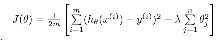
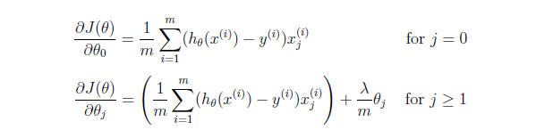
由于会产生Overffiting，所以本章节选用Regularized方法，进行优化。

具体 优化，参见下图。注意，多j=0的时候，没有进行。计算theta0的偏导的时候，要注意一下。

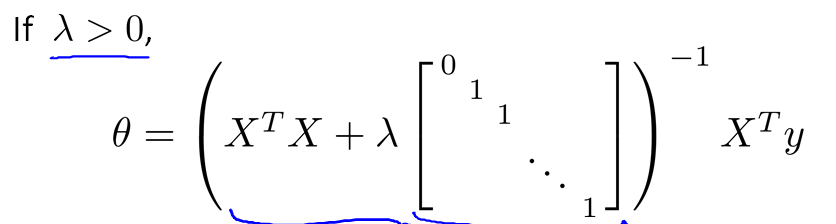
采用Normal Equation时候的，如果m<n,则regularized方法为

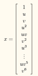
作业：在此问题中，不可以使用单独的一条直线分开两类。需要将特征x映射到一个28维的空间中，

其x向量映射后为：

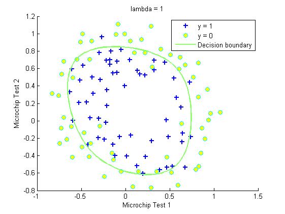
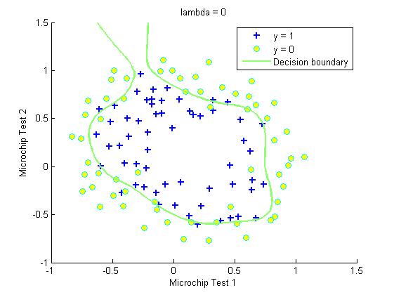
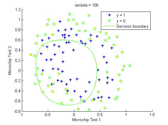
实验结果

clear ; close all; clc
data = load('ex2data2.txt');
X = data(:, [1, 2]); y = data(:, 3);
plotData(X, y);
hold on;
xlabel('Microchip Test 1')
ylabel('Microchip Test 2')
legend('y = 1', 'y = 0')
hold off;
%% =========== Part 1: Regularized Logistic Regression ============
X = mapFeature(X(:,1), X(:,2));


% Initialize fitting parameters
initial_theta = zeros(size(X, 2), 1);

% Set regularization parameter lambda to 1
lambda=1;

[cost, grad] = costFunctionReg(initial_theta, X, y, lambda);

%% ============= Part 2: Regularization and Accuracies =============

% Initialize fitting parameters
initial_theta = zeros(size(X, 2), 1);

% Set Options
options = optimset('GradObj', 'on', 'MaxIter', 400);


% Optimize
[theta, J, exit_flag] = ...
	fminunc(@(t)(costFunctionReg(t, X, y, lambda)), initial_theta, options);

% Plot Boundary
plotDecisionBoundary(theta, X, y);
hold on;
title(sprintf('lambda = %g', lambda))

xlabel('Microchip Test 1')
ylabel('Microchip Test 2')

legend('y = 1', 'y = 0', 'Decision boundary')
hold off;
p = predict(theta, X);
fprintf('Train Accuracy: %f\n', mean(double(p == y)) * 100);

下面来三个小函数

mapFeature和costFunction和plotDecisionBoundary

function [J, grad] = costFunctionReg(theta, X, y, lambda)

% Initialize some useful values
m = length(y); 

J = 0;
grad = zeros(size(theta));

theta_sub=theta(2:size(theta,1),:);
J=(y'*log(sigmoid(X*theta))+(1-y)'*log(1-sigmoid(X*theta)))/(-m)+theta_sub'*theta_sub*lambda/(2*m);
theta_g=[0;theta_sub];
grad=X'*(sigmoid(X*theta)-y)/m+lambda/m*theta_g;

end

function out = mapFeature(X1, X2)

%   Returns a new feature array with more features, comprising of 
%   X1, X2, X1.^2, X2.^2, X1*X2, X1*X2.^2, etc..
degree = 6;
out = ones(size(X1(:,1)));
for i = 1:degree
    for j = 0:i
        out(:, end+1) = (X1.^(i-j)).*(X2.^j);
    end
end
end