


1, subplot的使用
- matlab中的用法: subplot(m,n,p)或者subplot(m n p)
subplot是将多个图画到一个平面上的工具。其中,m和n代表在一个图像窗口中显示m行n列个图像,也就是整个figure中有n个图是排成一行的,一共m行,后面的p代表现在选定第p个图像区域,即在第p个区域作图。如果m=2就是表示2行图。p表示图所在的位置,p=1表示从左到右从上到下的第一个位置。
'''
注:ezplot(f,[-3,3]),表示画f函数的图形,取值区间在[-3,3]
代码如下:
'''
subplot(2,2,[1,2])
ezplot('sin',[-1,1])
grid minor
subplot(2,2,3)
ezplot('x',[-3,3])
subplot(2,2,4)
ezplot('x.^3',[-3,3])
grid- matplotlib 中的subplot的用法: subplot(numRows, numCols, plotNum)
python Matplotlib 可视化总结归纳(二) 绘制多个图像单独显示&多个函数绘制于一张图_haikuotiankong7的博客-CSDN博客_python的plot画多张图
Matplotlib的子图subplot的使用Matplotlib的子图subplot的使用 - 简书
matplotlib 中的subplot的用法matplotlib 中的subplot的用法 - 学弟1 - 博客园
import matplotlib.pyplot as plt
import numpy as np

def f(t):
    return np.exp(-t) * np.cos(2 * np.pi * t)

if __name__ == '__main__' :
    t1 = np.arange(0, 5, 0.1)
    t2 = np.arange(0, 5, 0.02)

    plt.figure(12)
    plt.subplot(221)
    plt.plot(t1, f(t1), 'bo', t2, f(t2), 'r--')

    plt.subplot(222)
    plt.plot(t2, np.cos(2 * np.pi * t2), 'r--')

    plt.subplot(212)
    plt.plot([1, 2, 3, 4], [1, 4, 9, 16])

    plt.show()
2,颜色反转Grayscale conversion和cmap的取值
plt.imshow(data, cmap='Greens') #cmap是colormap的简称,用于指定渐变色,默认的值为viridis, 在matplotlib中,内置了一系列的渐变色."""
==================
Colormap reference:https://matplotlib.org/examples/color/colormaps_reference.html
==================
Reference for colormaps included with Matplotlib.
This reference example shows all colormaps included with Matplotlib. Note that
any colormap listed here can be reversed by appending "_r" (e.g., "pink_r").
These colormaps are divided into the following categories:
Sequential:
These colormaps are approximately monochromatic colormaps varying smoothly
between two color tones---usually from low saturation (e.g. white) to high
saturation (e.g. a bright blue). Sequential colormaps are ideal for
representing most scientific data since they show a clear progression from
low-to-high values.
Diverging:
These colormaps have a median value (usually light in color) and vary
smoothly to two different color tones at high and low values. Diverging
colormaps are ideal when your data has a median value that is significant
(e.g. 0, such that positive and negative values are represented by
different colors of the colormap).
Qualitative:
These colormaps vary rapidly in color. Qualitative colormaps are useful for
choosing a set of discrete colors. For example::
color_list = plt.cm.Set3(np.linspace(0, 1, 12))
gives a list of RGB colors that are good for plotting a series of lines on
a dark background.
Miscellaneous:
Colormaps that don't fit into the categories above.
"""
import numpy as np
import matplotlib.pyplot as plt
# Have colormaps separated into categories:
# http://matplotlib.org/examples/color/colormaps_reference.html
cmaps = [('Perceptually Uniform Sequential', [
'viridis', 'plasma', 'inferno', 'magma']),
('Sequential', [
'Greys', 'Purples', 'Blues', 'Greens', 'Oranges', 'Reds',
'YlOrBr', 'YlOrRd', 'OrRd', 'PuRd', 'RdPu', 'BuPu',
'GnBu', 'PuBu', 'YlGnBu', 'PuBuGn', 'BuGn', 'YlGn']),
('Sequential (2)', [
'binary', 'gist_yarg', 'gist_gray', 'gray', 'bone', 'pink',
'spring', 'summer', 'autumn', 'winter', 'cool', 'Wistia',
'hot', 'afmhot', 'gist_heat', 'copper']),
('Diverging', [
'PiYG', 'PRGn', 'BrBG', 'PuOr', 'RdGy', 'RdBu',
'RdYlBu', 'RdYlGn', 'Spectral', 'coolwarm', 'bwr', 'seismic']),
('Qualitative', [
'Pastel1', 'Pastel2', 'Paired', 'Accent',
'Dark2', 'Set1', 'Set2', 'Set3',
'tab10', 'tab20', 'tab20b', 'tab20c']),
('Miscellaneous', [
'flag', 'prism', 'ocean', 'gist_earth', 'terrain', 'gist_stern',
'gnuplot', 'gnuplot2', 'CMRmap', 'cubehelix', 'brg', 'hsv',
'gist_rainbow', 'rainbow', 'jet', 'nipy_spectral', 'gist_ncar'])]
nrows = max(len(cmap_list) for cmap_category, cmap_list in cmaps)
gradient = np.linspace(0, 1, 256)
gradient = np.vstack((gradient, gradient))
def plot_color_gradients(cmap_category, cmap_list, nrows):
fig, axes = plt.subplots(nrows=nrows)
fig.subplots_adjust(top=0.95, bottom=0.01, left=0.2, right=0.99)
axes[0].set_title(cmap_category + ' colormaps', fontsize=14)
for ax, name in zip(axes, cmap_list):
ax.imshow(gradient, aspect='auto', cmap=plt.get_cmap(name))
pos = list(ax.get_position().bounds)
x_text = pos[0] - 0.01
y_text = pos[1] + pos[3]/2.
fig.text(x_text, y_text, name, va='center', ha='right', fontsize=10)
# Turn off *all* ticks & spines, not just the ones with colormaps.
for ax in axes:
ax.set_axis_off()
for cmap_category, cmap_list in cmaps:
plot_color_gradients(cmap_category, cmap_list, nrows)
plt.show()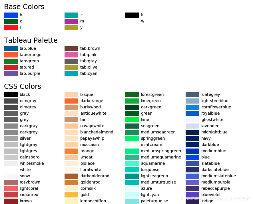
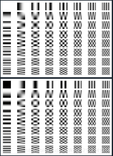
下面第一幅是用Greys, 第二幅是用Greys_r :
3,matplotlib.pyplot.axis()用法
axis()的用法axis()的用法 - 白羊呼啦 - 博客园
axis函数的使用(equal,ij,xy,tight,off,fill,normal.....)_蝉之洞-CSDN博客
matplotlib.pyplot.axis() matplotlib.pyplot.axis()与matplotlib.pyplot.axes()结构及用法_漫步量化-CSDN博客
4,matplotlib中的plt.figure()、plt.subplot()、plt.subplots()、add_subplots以及add_axes的使用
注意:subplot和subplots的区别
matplotlib中的plt.figure()、plt.subplot()、plt.subplots()、add_subplots以及add_axes的使用_小C的博客-CSDN博客
python3_matplotlib_figure()函数解析python3_matplotlib_figure()函数解析_也许有一天我们再相逢 睁开眼睛看清楚 我才是英雄!-CSDN博客
python中关于matplotlib库的figure,add_subplot,subplot,subplots函数python中关于matplotlib库的figure,add_subplot,subplot,subplots函数_墨羽羔羊的博客-CSDN博客_figure.add_subplot
5,python3,matplotlib绘图,title、xlabel、ylabel、图例等出现中文乱码
python3,matplotlib绘图,title、xlabel、ylabel、图例等出现中文乱码_why-csdn的博客-CSDN博客
在Windows系统找到中文字体添加进去就可以,只有部分字体能够右键查看他们的属性:C:\Windows\Fonts
'''
常用字体对应路径
宋体常规 C:\Windows\Fonts\simsun.ttc
新宋体常规 C:\Windows\Fonts\simsun.ttc
黑体常规 C:\Windows\Fonts\simhei.ttf
楷体常规 C:\Windows\Fonts\simkai.ttf
仿宋常规 C:\Windows\Fonts\simfang.ttf
隶体常规 C:\Windows\Fonts\SIMLI.TTF
华文新魏 C:\Windows\Fonts\STXINWEI.TTF
'''
'''
%matplotlib inline 可以在Ipython编译器里直接使用,功能是可以内嵌绘图,并且可以省略掉plt.show()这一步。
但在spyder用会报错. 经过我的的验证该句在spyder下的Ipython也没有任何作用,因为在spyder下的Ipython会自动输出图像
'''
%matplotlib inline
import matplotlib # 注意这个也要import一次
import matplotlib.pyplot as plt
#from matplotlib.font_manager import FontProperties
#font_set = FontProperties(fname=r"c:/windows/fonts/simsun.ttc", size=15)
'''
路径中的双引号和单引号都可以,斜杠和反斜杠也都可以
另外说明:因python3默认使用中unicode编码, 所以在写代码时不再需要写 plt.xlabel(u'横'),而是直接写plt.xlabel('横')
'''
#myfont = matplotlib.font_manager.FontProperties(fname=r"C:\Windows\Fonts\STXINWEI.TTF") # fname指定字体文件 选简体显示中文
myfont = matplotlib.font_manager.FontProperties(fname=r'C:\Windows\Fonts\simkai.ttf', size=15)
plt.plot((1,2,3),(4,3,-1))
plt.xlabel('横', fontproperties=myfont) # 这一段
plt.ylabel('纵', fontproperties=myfont) # 这一段
#plt.show() # 有了%matplotlib inline 就可以省掉plt.show()了
'''
也可以不使用matplotlib.font_manager.FontProperties语句导入字体,直接使用fontproperties='SimHei',matplotlib可以自己找到部分字体,但找不全
'''
plt.plot((1,2,3),(4,3,-1))
plt.xlabel(u'横坐标', fontproperties='STXINWEI') #新魏字体
plt.ylabel(u'纵坐标', fontproperties='SimHei') # 黑体
6,matplotlib基础绘图命令之imshow
matplotlib基础绘图命令之imshow - 云+社区 - 腾讯云
7,用箭头和文字来标记重要的点,对图标的坐标轴进行调整
8,python画图入门汇总教程-先看
Python3快速入门(十六)——Matplotlib绘图Python3快速入门(十六)——Matplotlib绘图_生命不息,奋斗不止的技术博客_51CTO博客_matplotlib绘图教程
python画图入门python画图入门 - 知乎
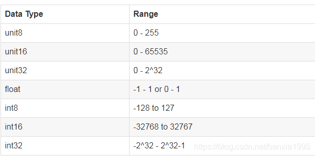
9,python:图片的float类型和uint8类型
python:图片的float类型和uint8类型_宁静致远*的博客-CSDN博客
python中不同函数读取图片格式的区别python中不同函数读取图片格式的区别_u013044310的博客-CSDN博客_img.astype
在python图像处理过程中,遇到的RGB图像的值是处于0-255之间的,为了更好的处理图像,通常python提供的读取图片函数默认都会将图像值转变到0-1之间.
float,float32,float64这三个数据类型的范围都是 [0.0, 1.0] or [-1.0, 1.0] :Module: util — skimage v0.18.0 docs
10,scipy.misc.bytescale的替代方案
scipy.misc.bytescale的替代函数代码scipy.misc.bytescale.py-机器学习文档类资源-CSDN下载
skimage.util.img_as_ubyteis a replacement forscipy.misc.bytescalethe scipy.misc.bytescale doc states the following:
Byte scaling means converting the input image to uint8 dtype and scaling the range to (low, high) (default 0-255). If the input image already has dtype uint8, no scaling is done.
the skimage.util.img_as_ubyte doc states the following:
Convert an image to 8-bit unsigned integer format. Negative input values will be clipped. Positive values are scaled between 0 and 255.
python - What replaces scipy.misc.bytescale? - Stack Overflow
python - Alternatives to Scipy's misc bytescale method - Stack Overflow
11,matplotlib.pyplot.imread函数返回值
matplotlib.pyplot.imread — Matplotlib 3.1.2 documentation
| Returns: | imagedata : The image data. The returned array has shape
|
|---|
12,用python将图像转换为三维数组
RGB images are usually stored as 3 dimensional arrays of 8-bit unsigned integers. The shape of the array is:
height x width x 3. 这和分辨率(1920×1080)恰相反
用python将图像转换为三维数组之后,每一维,每个元素值都代表着什么?用python将图像转换为三维数组之后,每一维,每个元素值都代表着什么?_向东的笔记本-CSDN博客
13, Creating Image with numpy
在线拾色器-输入RGB值输出颜色在线拾色器 - W3Cschool
14,numpy之histogram,plt.bar()与plt.barh条形图
numpy之histogram_Nicola.Zhang-CSDN博客
plt.bar()与plt.barh条形图4.4Python数据处理篇之Matplotlib系列(四)---plt.bar()与plt.barh条形图 - 梦并不遥远 - 博客园
numpy.histogram(a, bins=10, range=None, normed=False, weights=None, density=None)[source]
Returns: hist : array
The values of the histogram. See density and weights for a description of the possible semantics.
bin_edges : array of dtype float
Return the bin edges
(length(hist)+1)
a是待统计数据的数组;
bins指定统计的区间个数;
range是一个长度为2的元组,表示统计范围的最小值和最大值,默认值None,表示范围由数据的范围决定
weights为数组的每个元素指定了权值,histogram()会对区间中数组所对应的权值进行求和
density为True时,返回每个区间的概率密度;为False,返回每个区间中元素的个数
import numpy as np
import matplotlib.pyplot as plt

a = np.random.rand(100)
np.histogram(a,bins=5,range=(0,1))
dct_hist, dct_bin_edges = np.histogram(a,bins=5,range=(0,1))
img_hist, img_bin_edges = np.histogram(a,bins=[0,0.2,0.5,0.8,1])

f, (plt1, plt2) = plt.subplots(1, 2, figsize=(15, 5))

plt1.set_title('Frequency histogram')
plt1.bar(dct_bin_edges[:-1], dct_hist, width = 0.1)#注意dct_bin_edges的数据比dct_hist数据多一个,因此要去除一个数据才能画图

plt2.set_title('Spatial histogram')
plt2.bar(img_bin_edges[1:], img_hist, width = 0.1)

#输出
In [75]: np.histogram(a,bins=5,range=(0,1))
Out[75]:
(array([18, 19, 13, 24, 26], dtype=int64),#注意bin_edges的数据比hist数据多一个,即the bin edges (length(hist)+1)
 array([0. , 0.2, 0.4, 0.6, 0.8, 1. ]))   #18表示a中有18个数落在[0,0.2]区间,19个数落在[0.2,0.4]区间

In [76]: np.histogram(a,bins=[0,0.2,0.5,0.8,1])
Out[76]: (array([18, 26, 30, 26], dtype=int64), array([0. , 0.2, 0.5, 0.8, 1. ]))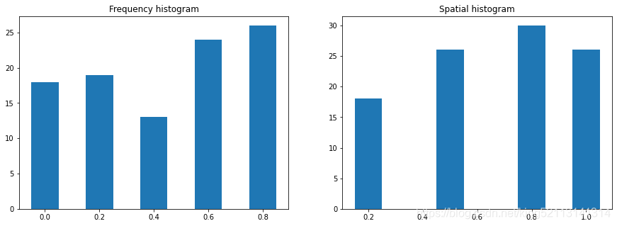
15,Python中[ : n]、[m : ]、[-1]、[:-1]、[::-1]、[2::-1]和[1:]的含义
Python中[ : n]、[m : ]、[-1]、[:-1]、[::-1]、[2::-1]和[1:]的含义_SpringRolls的博客-CSDN博客_python是什么意思
Python中双冒号的作用[::]
Python sequence slice addresses can be written as a[start:end:step] and any of start, stop or end can be dropped.
Python序列切片地址可以写为[开始:结束:步长],其中的开始和结束可以省略
16,Python数据可视化(一):散点图绘制
Custom a Matplotlib Scatterplot
17,颜色,线条,标志形状
matplotlib横坐标从大到小_Python数据分析:Matplotlib_weixin_39958631的博客-CSDN博客
matplotlib.pyplot.plot — Matplotlib 3.4.3 documentation
18,画子图
https://www.jb51.net/article/254132.htm
一次性掌握所有 Python 画图基础操作_Gene_INNOCENT的博客-CSDN博客_python画图
Python图像绘制基础——子图绘制_银河初升的博客-CSDN博客_python 子图
import numpy as np
import matplotlib
import matplotlib.pyplot as plt
from matplotlib import style

style.use('ggplot')  # 加载'ggplot'风格
matplotlib.rcParams['text.usetex'] = True  # 开启Latex风格
plt.figure(figsize=(10, 10), dpi=70)  # 设置图像大小
f, ax = plt.subplots(2, 2)  # 设置子图


def func1():
    X = np.linspace(0, 1, 100)
    Y1 = np.sqrt(X)
    # ax[0][0]的设置
    ax[0][0].plot(X, Y1, color="lightcoral", linewidth=3.0, linestyle="-", label=r"$y_1=\sqrt{x}$")
    ax[0][0].set_xlabel('x', fontsize=10)
    ax[0][0].set_ylabel('y', fontsize=10)
    ax[0][0].set_title(r'$f(x)=\sqrt{x}$', fontsize=16)
    ax[0][0].legend(loc="best")

    # ax[0][0]关键点
    ax[0][0].scatter(0.5, np.sqrt(0.5), s=100)
    ax[0][0].annotate("End Point",
                      xy=(0.6, 0.5),
                      fontsize=12,
                      xycoords="data")


def func2():
    X = np.linspace(0, 1, 100)
    Y2 = X
    # ax[0][1]的设置
    ax[0][1].plot(X, Y2, color="burlywood", linewidth=3.0, linestyle="--", label=r"$y_2=x$")
    ax[0][1].set_xlabel('x', fontsize=10)
    ax[0][1].set_ylabel('y', fontsize=10)
    ax[0][1].set_title(r'$f(x)=x$', fontsize=16)
    ax[0][1].legend(loc="best")

    # ax[0][1]关键点
    ax[0][1].scatter(0.5, 0.5, s=100)
    ax[0][1].annotate("End Point",
                      fontsize=12,
                      xytext=(0.7, 0.1),
                      xy=(0.5, 0.5),
                      xycoords="data",
                      arrowprops=dict(facecolor='gray', shrink=0.15))


def func3():
    X = np.linspace(0, 1, 100)
    Y3 = X * X
    # ax[1][0]的设置
    ax[1][0].plot(X, Y3, color="mediumturquoise", linewidth=3.0, linestyle="-.", label=r"$y_3=x^2$")
    ax[1][0].set_xlabel('x', fontsize=10)
    ax[1][0].set_ylabel('y', fontsize=10)
    ax[1][0].set_title(r'$f(x)=x^2$', fontsize=16)
    ax[1][0].legend(loc="best")

    # ax[1][0]关键点
    ax[1][0].scatter(0.5, 0.5 * 0.5, s=100)
    ax[1][0].annotate("End Point",
                      fontsize=12,
                      xytext=(0.05, 0.6),
                      xy=(0.5, 0.5 * 0.5),
                      xycoords="data",
                      arrowprops=dict(facecolor='black', shrink=0.1))


def func4():
    X = np.linspace(0, 1, 100)
    Y4 = X * X * X
    # ax[1][1]的设置
    ax[1][1].plot(X, Y4, color="mediumpurple", linewidth=3.0, linestyle=":", label=r"$y_4=x^3$")
    ax[1][1].set_xlabel('x', fontsize=10)
    ax[1][1].set_ylabel('y', fontsize=10)
    ax[1][1].set_title(r'$f(x)=x^3$', fontsize=16)
    ax[1][1].legend(loc="best")

    # ax[1][1]关键点
    ax[1][1].scatter(0.5, 0.5 * 0.5 * 0.5, s=100)
    ax[1][1].annotate("End Point",
                      xy=(0.2, 0.3),
                      fontsize=12,
                      xycoords="data")


def main():
    func1()
    func2()
    func3()
    func4()

    plt.tight_layout()  # 当有多个子图时,可以使用该语句保证各子图标题不会重叠
    plt.savefig('myplot1.pdf', dpi=700)  # dpi 表示以高分辨率保存一个图片文件,pdf为文件格式,输出位图文件
    plt.show()


if __name__ == "__main__":
    main()


################也可以使用 plt.sca() 来定位子图,如下述例子:
f, ax = plt.subplots(2, 3, figsize=(15, 10)) # 声明 2 行 3 列的子图
f.suptitle("设置总标题", fontsize=18)

plt.sca(ax[0, 1]) # 定位到第 1 行第 2 列的子图
# 接下来直接使用 plt 画图即可
19,箱图
【迅速上手】Python 画图 —— 箱图与密度图_Gene_INNOCENT的博客-CSDN博客
20,基础知识
Python 各种画图_流浪猪头拯救地球的博客-CSDN博客_python画图
import matplotlib.pyplot as plt			# 导入模块

plt.style.use('ggplot')					# 设置图形的显示风格
fig=plt.figure(1)						# 新建一个 figure1
fig=plt.figure(figsize=(12,6.5),dpi=100,facecolor='w')
fig.patch.set_alpha(0.5)				# 设置透明度为 0.5
font1 = {'weight' : 60, 'size' : 10}	# 创建字体,设置字体粗细和大小
ax1.set_xlim(0,100)						# 设置 x 轴最大最小刻度
ax1.set_ylim(-0.1,0.1)					# 设置 y 轴最大最小刻度
plt.xlim(0,100)  						# 和上面效果一样
plt.ylim(-1,1)
ax1.set_xlabel('X name',font1)			# 设置 x 轴名字
ax1.set_ylabel('Y name',font1)			# 设置 y 轴名字
plt.xlabel('aaaaa')						# 设置 x 轴名字
plt.ylabel('aaaaa')						# 设置 y 轴名字
plt.grid(True)					 		# 增加格网
plt.grid(axis="y")						# 只显示横向格网
plt.grid(axis="x")						# 只显示纵向格网
ax=plt.gca()							# 获取当前axis,
fig=plt.gcf()							# 获取当前figures
plt.gca().set_aspect(1)					# 设置横纵坐标单位长度相等
plt.text(x,y,string)					# 在 x,y 处加入文字注释
plt.gca().set_xticklabels(labels, rotation=30, fontsize=16) # 指定在刻度上显示的内容
plt.xticks(ticks, labels, rotation=30, fontsize=15)   # 上面两句合起来
plt.legend(['Float'],ncol=1,prop=font1,frameon=False)	# 设置图例 列数、去掉边框、更改图例字体
plt.title('This is a Title')			# 图片标题
plt.show()								# 显示图片,没这行看不见图
plt.savefig(path, dpi=600)				# 保存图片,dpi可控制图片清晰度
plt.rcParams['font.sans-serif'] = ['SimHei']  	# 添加这条可以让图形显示中文
mpl.rcParams['axes.unicode_minus'] = False		# 添加这条可以让图形显示负号
ax.spines['right'].set_color('none')
ax.spines['top'].set_color('none')				#设置图片的右边框和上边框为不显示
# 子图
ax1=plt.subplot(3,1,1)
ax1.scatter(time,data[:,1],s=5,color='blue',marker='o') # size, color, 标记
ax1=plt.subplot(3,1,2)
...
# 控制图片边缘的大小
plt.subplots_adjust(left=0, bottom=0, right=1, top=1,hspace=0.1,wspace=0.1)

# 设置坐标刻度朝向,暂未成功
plt.rcParams['xtick.direction'] = 'in'
ax = plt.gca()
ax.invert_xaxis()
ax.invert_yaxis()
参考:
python数字图像处理 https://www.cnblogs.com/denny402/p/5121501.html
python skimage图像处理(一)python skimage图像处理(一) - 简书
用python简单处理图片(1):打开\显示\保存图像 用python简单处理图片(1):打开\显示\保存图像 - denny402 - 博客园
「Matplotlib绘图详解」史上最全Matplotlib教程 - 知乎
Matplotlib 教程Matplotlib 教程 | 菜鸟教程
Matplotlib official tutorial https://matplotlib.org/tutorials/colors/colormaps.html
python之matplotlib绘图基础 python之matplotlib绘图基础 - tongqingliu - 博客园


 4133
4133


 被折叠的 条评论
为什么被折叠?
被折叠的 条评论
为什么被折叠?
 到【灌水乐园】发言


