Building a Recommendation Engine with Spark and EMR

Building a recommendation engine from scratch has been a difficult but rewarding experience. I wanted to incorporate song recommendations based on users’ listening habits in 33 RPM (update: sadly no longer in service).

Originally, 33 RPM’s recommendations were generated by comparing users’ historical play data with the entire catalog of songs that are stored using a combination of Euclidian distance and Jaccard Index algorithms. The generated results were satisfactory, but it was extremely slow. It took roughly one hour to generate recommendations per user, and it would only increase as the catalog grew.

I looked into alternatives and came across Apache Spark which has many machine learning libraries, one of which can be used to create a recommendation engine. After switching to Spark and getting it up and running on AWS EMR, recommendations are now generated in five to ten minutes and I’m very happy with the results I’ve seen.

I had a lot of fun learning about Spark, but it was kind of frustrating too – a lot of resources and documentation I’ve found is outdated. Did you know Spark has two ML libraries? ML and MLlib, the latter of which is deprecated but the majority of examples online still use. So I wanted to create a guide and outline the steps I took using the latest version of Spark (2.2.0) and ML.

How are recommendations generated, anyway?

There are three main approaches when implementing a recommendation engine:

• Content-based Filtering
• Collaborative Filtering
• A combination of both

Content-based filtering uses metadata or properties about the items you want to recommend. For example: genres, tempo, and valence could be used to recommend songs by comparing the songs you’ve played against songs you haven’t played and measuring the similarities of these values (similar to the approach I was using originally).

Collaborative filtering takes a different approach and compares similarity amongst users. An extremely simplified example of this is if I listened to {Song A, Song B} and you listened to {Song B, Song C} I would get recommended Song C and you would get recommended Song A.

I decided to go with collaborative filtering for a couple of reasons: the results I saw using collaborative filtering were (subjectively) better, and while I can get metadata for most songs, there are a lot of songs that fail to retrieve metadata for a variety reasons thus limiting the pool for potential recommendations.

Spark includes a collaborative filtering library using the alternating least squares (ALS) algorithm. ALS is type of matrix factorization which generates a large matrix of users and items (or “purchases”, using the diagram below) and factors the matrix into two smaller matrices for users and products called latent factors. The algorithm then predicts missing entries within these factors.

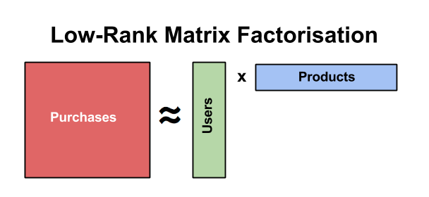
Source: http://danielnee.com/2016/09/collaborative-filtering-using-alternating-least-squares/

That’s just a very basic explanation of ALS, but you can read more about it here if you’re interested.

Implicit vs. Explicit Feedback

When using collaborative filtering, you can choose to train your model with either implicit feedback or explicit feedback. Implicit feedback is usually something like views, clicks, purchases, etc. while explicit feedback is usually a user-supplied rating. Per the documentation regarding Implicit vs. Explicit feedback:

Essentially, instead of trying to model the matrix of ratings directly, this approach treats the data as numbers representing the strength in observations of user actions (such as the number of clicks, or the cumulative duration someone spent viewing a movie). Those numbers are then related to the level of confidence in observed user preferences, rather than explicit ratings given to items. The model then tries to find latent factors that can be used to predict the expected preference of a user for an item.

In our case, we’re going to treat whether or not a user has played a song as implicit feedback.

Setting up Spark

Spark can be easily installed with Homebrew:

brew update
brew install apache-spark

You’ll also want to set the SPARK_HOME env variable with the installation path:

export SPARK_HOME=/usr/local/Cellar/apache-spark/2.2.0/libexec

Start Spark by running the following commands:

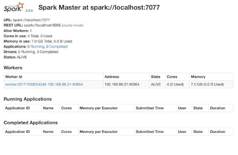
$SPARK_HOME/sbin/start-master.sh --host localhost
$SPARK_HOME/sbin/start-slave.sh --master spark://localhost:7077

Now you should be able to access the Spark UI by visiting localhost:8080.

Setting up Jupyter Notebook

I highly recommend using Jupyter Notebook as a way to “sketch out” your ideas and immediately test and evaluate your Spark applications using python. Jupyter can be installed using pip:

pip install findspark jupyter

We’re installing findspark as well which adds PySpark to your path at runtime.

Start jupyter with the following command:

jupyter notebook

This will open a new tab in your browser. Select New > Python 2 and let’s get to it!

Preparing Our Data

First, we’re going to call findspark.init() to ensure the PySpark libraries are loaded into the path at runtime and then we’ll create a new SparkSession:

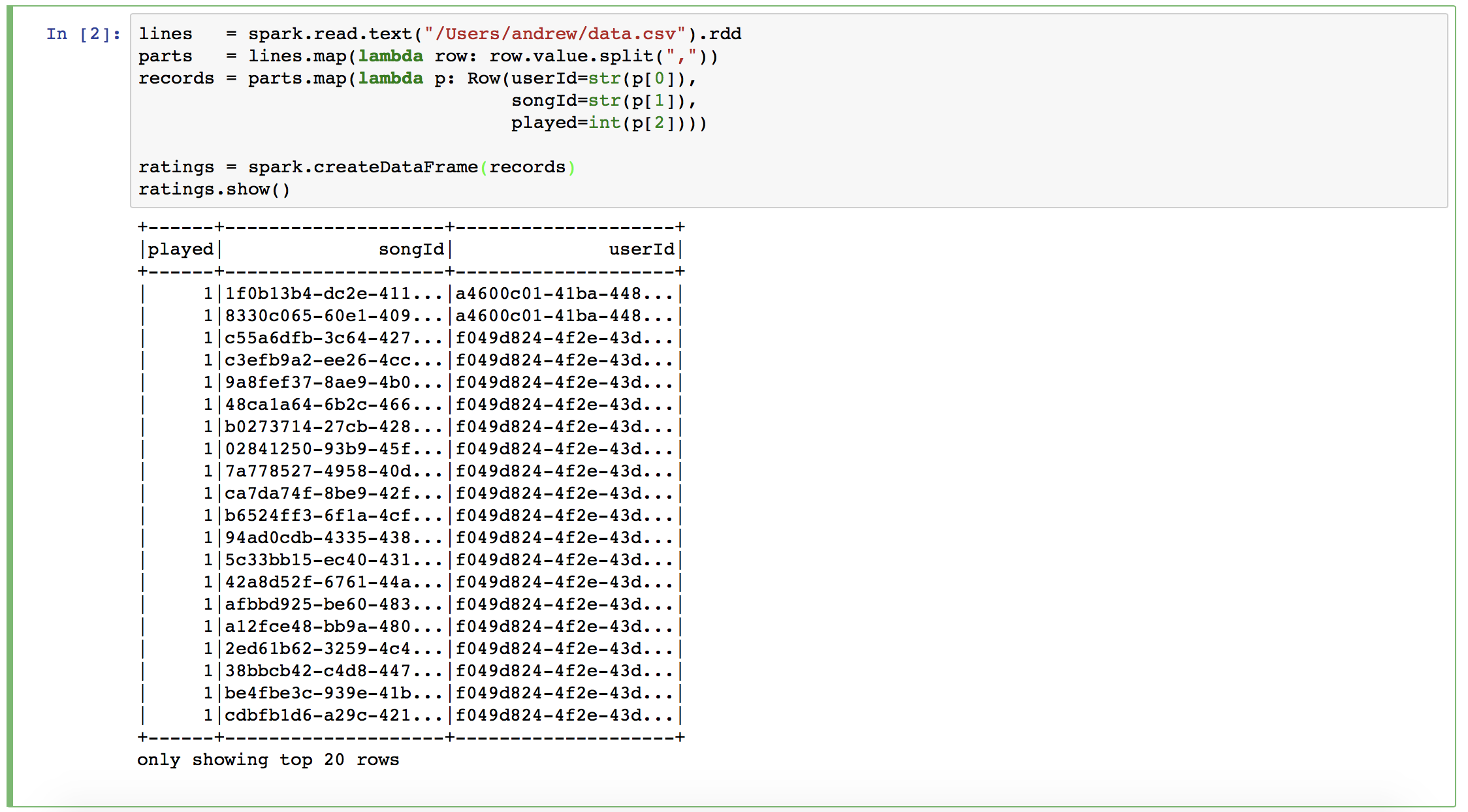
Next, we’re going to read from a csv file to create a DataFrame of rows. A DataFrame is a distributed collection of data organized into named columns and is conceptually similar to a table in a relational database.

This DataFrame contains song IDs, user IDs, and a “played” attribute which is set to 1. This attribute is considered to be our implicit feedback and we’re going to tell our model to treat it as such in a couple of steps.

One small problem: the data used to train our model can only have integer or double values, but here we have string UUIDs. To get around this we can use Spark’s provided StringIndexer function to encode our strings into indices ordered by frequency. A StringIndexer can only be used for one column, so we’re also going to use a Pipeline to combine them.

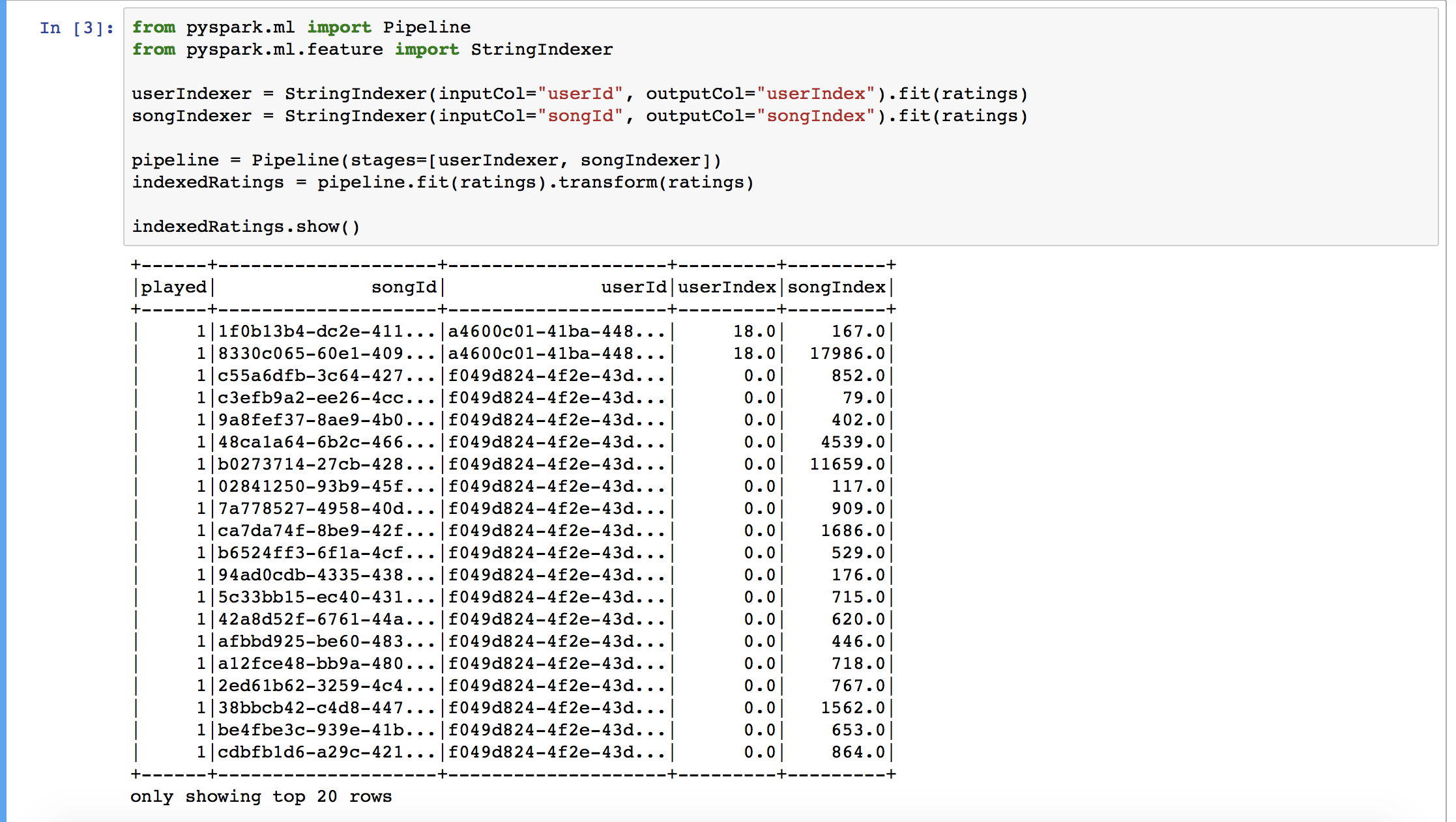
Now we have two new columns (userIndex and songIndex) which we can use to train our ML model.

Training and Evaluating

Now we can start training and evaluating our model. This requires a lot of tinkering and playing around with different values to get the lowest Root-mean-square error (RMSE). Measuring the RMSE is a common method of testing the accuracy of a model’s predictions. We can do this by randomly splitting up our data and use 80% of it for training and the other 20% for testing. The data used for testing will compare known values to the generated predictions to measure accuracy.

Using Spark’s RegressionEvaluator we can iterate through different ranks, alphas, iterations, etc. to find the lowest RMSE.

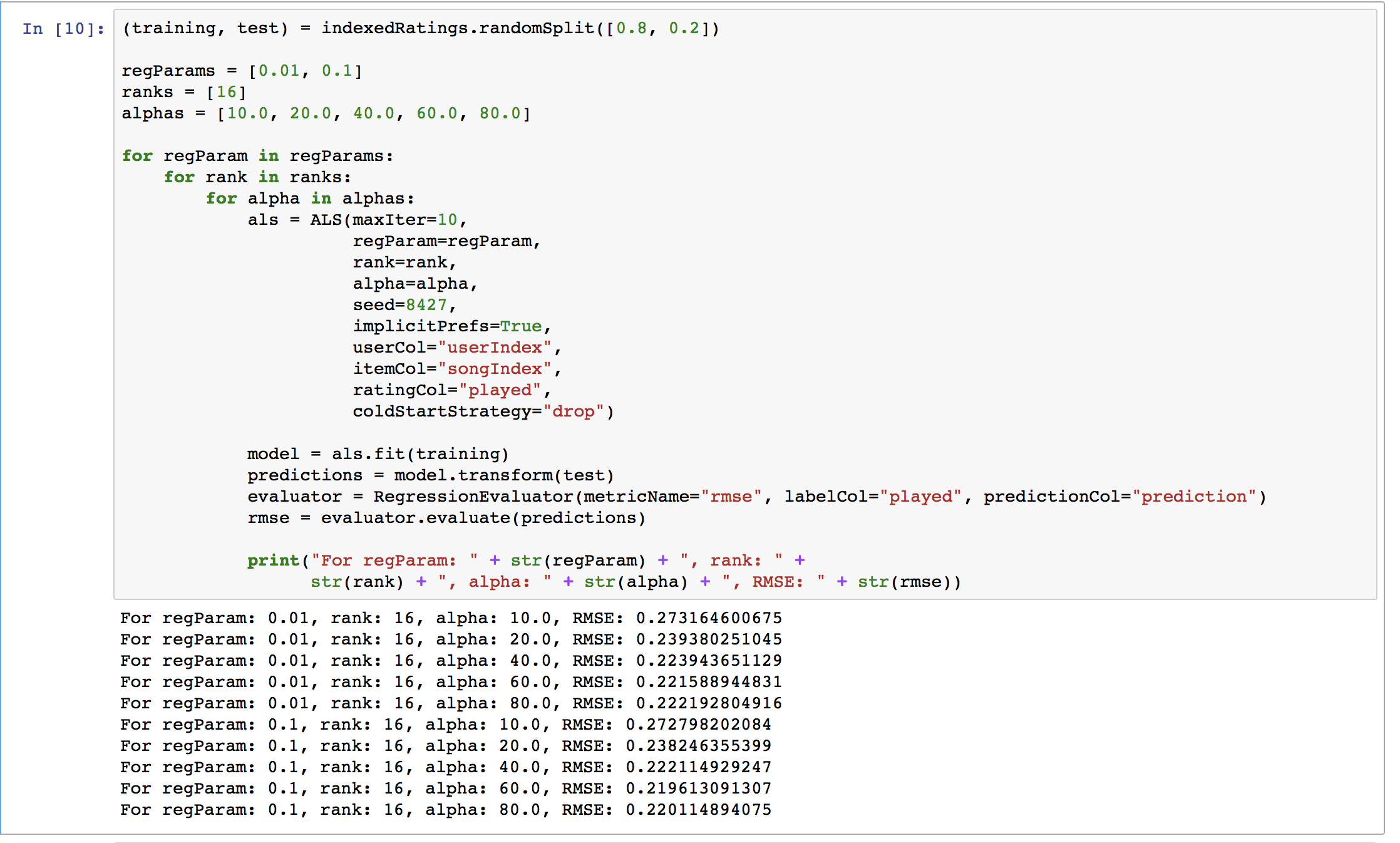
In this example, our lowest RMSE is 0.219* using a regularization parameter of 0.1, rank of 16, and alpha of 60.0.

Here’s a breakdown of the parameters used when creating the ALS object:

• maxIter – Maximum number of iterations to run (default: 10)
• regParam – Regularization parameter. Reduces overfitting your model which leads to the reduction of variance in estimates; however, it comes with the expense of adding more bias. (default: 0.01)
• rank – Size of the feature vectors to use. Larger ranks can lead to better models but are more expensive to compute (default: 10)
• alpha – A constant used for computing confidence with implicit datasets. (default: 1.0)
• seed – A constant used to make randomized algorithms behave deterministically, leading to repeatable results. (default: None) implicitPrefs – Set to True when working with implicit feedback. (default: False)
• userCol – Name of the column containing user IDs (default: user)
• itemCol – Name of the column containing item IDs (default: item)
• ratingCol – Name of the column containing the ratings (default: rating)
• coldStartStrategy – Strategy for dealing with unknown or new items/users. Setting it to “drop” simply excludes these items from the results. (default: nan)

Generating Recommendations

Now we can generate our recommendations. Let’s generate 10 recommendations per user.

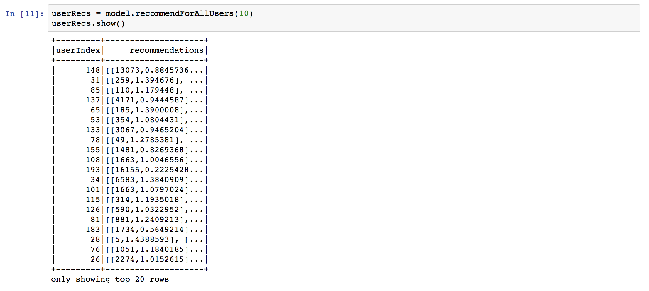
The data in the recommendations column is formatted as an array of structs containing <song id, rating>. Because we still need to convert the indexes back into UUID strings, I found it a lot easier to work with this data when flattening the recommendations. Using the withColumn and explode functions, we can transform the DataFrame and split the songs and scores into their own rows.

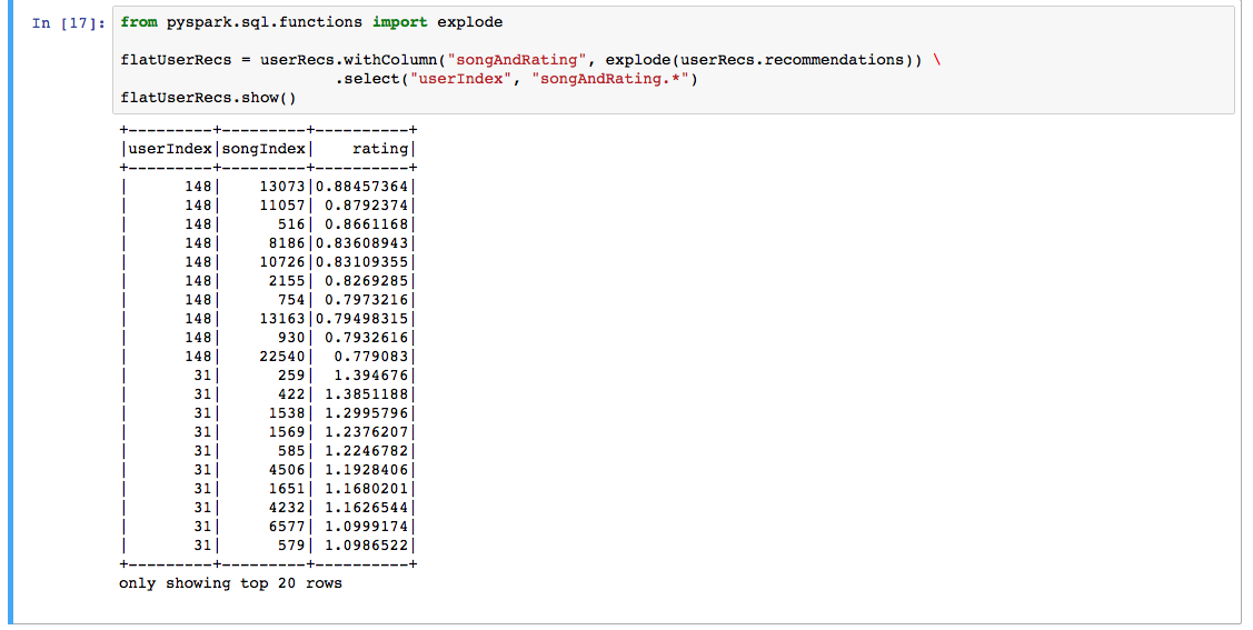
Ah, much better!

Now we can easily convert our indexes back into strings using IndexToString and another Pipeline.

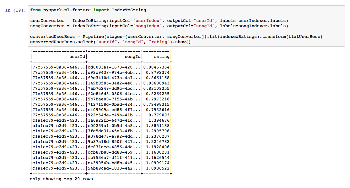
Check that out, you just created a machine learning recommendation engine!

Exporting the Results

Now we can save our data using the write function, which accepts many types of formats: CSV, JSON, etc.

This will create a results directory with several csv files because of Spark’s distributed nature. You can get around this by using the coalesce function, but be aware this method isn’t recommended when working with a large dataset.

Running Jobs with spark-submit

Now we’re ready to put everything we have into a python file and run our spark application using the spark-submit command. After you create your python file, you can use the following command:

$SPARK_HOME/bin/spark-submit --master spark://localhost:7077 recommender.py

If desired, you can also pass in arguments (after the py file) and parse them in your code using sys.argv.

AWS EMR

Running your Spark applications on AWS EMR is fairly simple and has native S3 file support thanks to Hadoop.

To read and write from S3 let’s change a couple of lines: the read line near the beginning of our program and the write line near the end.

lines   = spark.read.text("s3://bucket/file.csv").rdd
# ...
convertedUserRecs.write.csv("s3://bucket/results")

Head on over to the EMR console and create a new cluster. You have two launch modes to choose from:

• Cluster – spin up a long-lived cluster
• Step execution – spin up a cluster, run a specified task, and teardown the cluster upon completion

For this example let’s choose step execution.

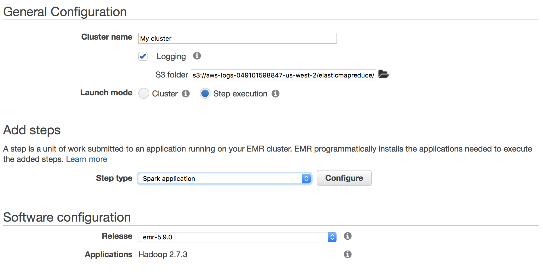
Choose “Spark application” from the step type dropdown and click “Configure”. This will bring up a modal to specify which file to run and specify any arguments if needed.

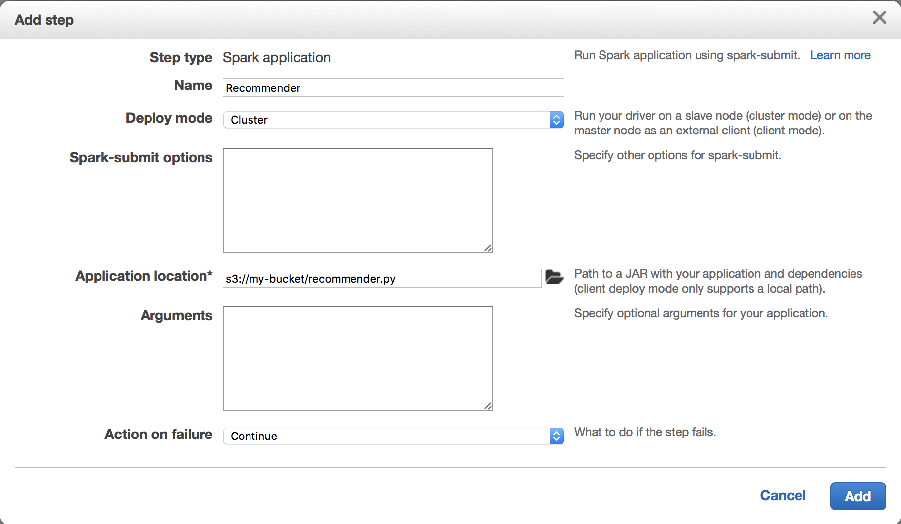
Click “Add” and then “Create Cluster”.

Your cluster will take a few minutes to spin up, but afterwards you can click the “Steps” tab to view progress of your Spark application.

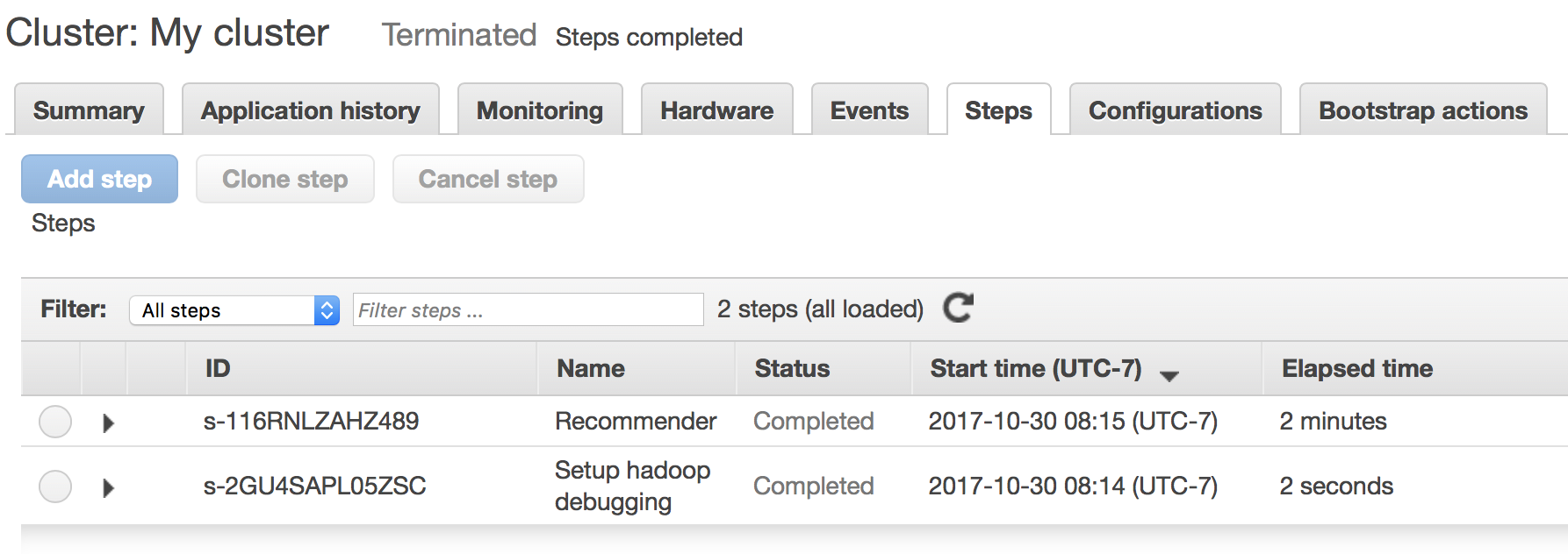
Hooray, our step completed successfully! Now we have our results saved in S3.

If you want to get fancy, you can set up an S3 Event Notification to trigger a Lambda function or send a message to an SQS queue to process your data after your EMR step is finished. You can also set up a Data Pipeline to copy data from a database into S3, spin up an EMR cluster to generate your recommendations, and export that data into a database (for example).

This just scratches the surface of what you can do with Spark and EMR, but I hope this post provided you with a good starting point!

Resources

• GitHub Repo
• Collaborative Filtering – Spark 2.2.0 Documentation
• Complete Guide on DataFrame Operations in PySpark
• Matrix Factorization Techniques for Recommender Systems
• Collaborative Filtering using Alternating Least Squares

转载：https://schaper.io/2017/10/building-a-recommendation-engine-with-spark-and-emr/