


 本文探讨了Greenplum数据库中的SQL查询优化技术,包括Pivotal Query Optimizer的使用、查询计划的理解以及如何利用内置函数和操作符提高查询效率。
24 查询数据
本主题提供有关在Greenplum的数据库使用SQL的信息。
你进入所谓的查询中使用PSQI交互式SQL客户端和其他客户端工具的数据库查看,更改和分析数据的SQL语句。
• 定义查询
• 使用函数和操作符
• 查询性能
• 查询剖析
24.1 关于 Greenplum查询处理
本主题提供Greenplum数据引擎如何处理查询的概述。了解这个过程在编写和调整查询时,可能非常有用。
用户和使用其他数据库系统一样来使用GPDB。他们可以通过PSQL或其他的客户端来连接到GPDB的master上并执行SQL。
24.1.1理解查询计划和调度
master 负责接收、分析,优化查询。由此产生的查询计划是并行的或有针对性的。Master分发给并行查询计划给所有的段,如图19所示。master调度一个目标查询到一个单节点,如图20所示。每个段通过在自己的本地数据库执行查询以响应查询需求。大多数的数据库操作,如表扫描,连接,聚合,排序等操作在所有的节点上并行执行。每个操作都在一个段数据上进行操作,和其他段的数据没有任何关联。
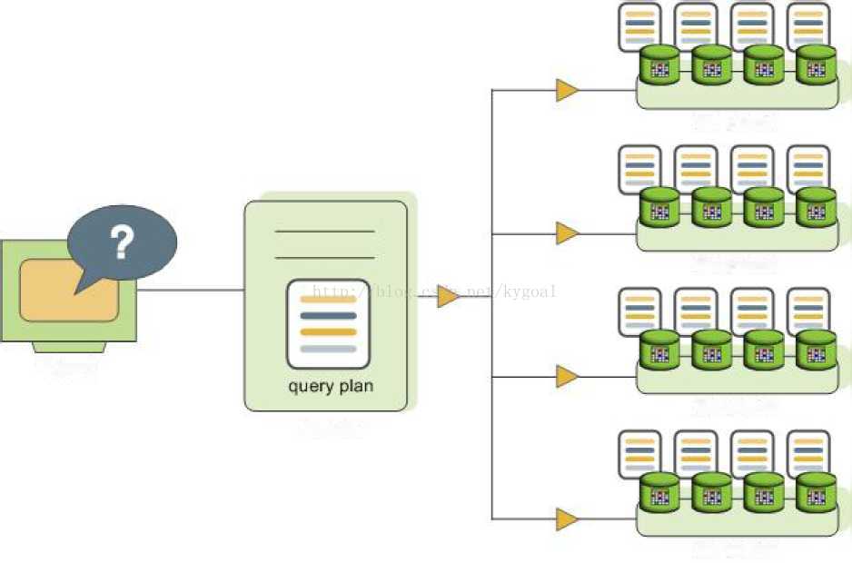
Figure 19: Dispatching the Parallel Query Plan
某些查询可能只访问单个段,如通过散列键过滤后的单行insert, update, delete, or select,这些查询不会分发到所有的节点上。但是会标记所有包含受影响或相关的行。In queries such as these,the query plan is not dispatched to all segments,but is targeted at the segment that contains the affected or relevant row(s).
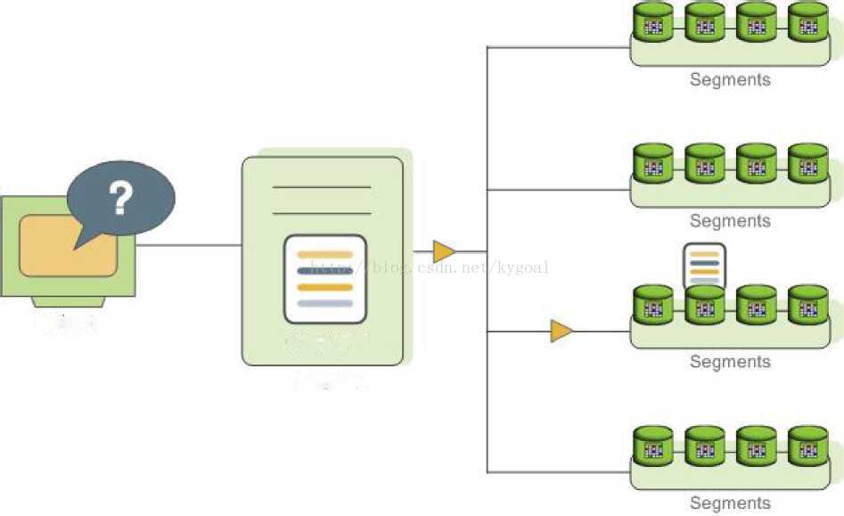
Figure 20: Dispatching a Targeted Query Plan
24.1.2理解Greenplum查询计划
查询计划是Greenplum数据引擎将要执行的一系列操作以获得查询结果的操作。计划中的每一个节点或一步代表一个数据库的操作,如表扫描,连接,聚集或排序。计划被读出并从下到上执行。
除了常见的数据库操作,如表扫描,联接等,Greenplum数据引擎有一个叫做motion额外的操作类型。移动操作涉及查询处理期间移动段之间的元组。请注意,并非所有的查询需要的数据移动。例如,有针对性的查询计划不要求数据在整个网络移动。
要实现查询执行过程中最大并行,Greenplum将查询计划的进行分片。每个分片是段可以独立工作的计划的一部分。无论在计划中发生运动操作,搭配上运动的每一侧一片查询计划切片。
例如,请考虑涉及两个表之间的连接下面的简单查询:
例如, consider the following simple query involving a join between two tables:
SELECT customer, amount
FROM sales JOIN customer USING (cust_id)
WHERE dateCol = '04-30-2008';
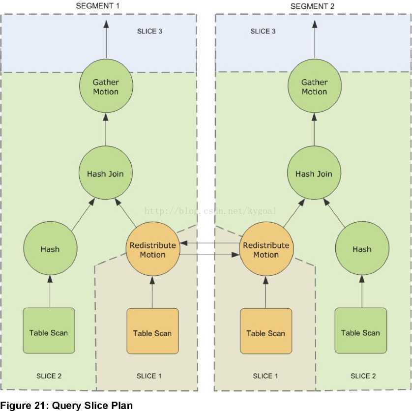
图21 21: Query Slice Plan展示了查询计划。每个段都接收了查询计划的副本,并在本地并行执行。在这里例子中,为了完成关联操作,需要执行重分布数据移动操作。重分布数据移动在这里是必要的,因为customer表是用cust_id来散列的,到sales表是用sale_id来散列的。为了执行管理,sales的元组必须按照cust_id进行重新分布。查询计划在数据分布移动的两侧创建了两个片,分别是slice 1 和 slice 2.这个查询计划还有另外一个数据移动操作,称为收集运行(gather motion)。收集运动是当段需要发送结果到master节点用于呈现给客户端时发生的。因为查询计划在数据移动时总要进行分片,因此这个查询加护就在顶端实现了另一个分片slice3。然而并不是所有的查询就会触发gather motion,例如acreate table x as select... 就不会产生一个gather motion因为元组都发送到新创建的表了,而不是master。
24.1.3理解查询并行执行
GPDB创建了一系列的数据库进程来执行查询操作。在master,这个查询工作进程被称为查询调度器query dispatcher (QD). 查询调度器负责创建和调度查询计划,并且聚合以及呈现最终结果。在段上,执行查询的工作进程被称为查询执行器 query executor (QE). 查询执行器负责完成给定的查询工作部分并且和其他工作进程进行中间结果的交流。
对查询计划的每个分片,至少有一个工作进程被分配给它。一个工作进程独立运行查询计划分配给它的部分。在查询执行过程中,每个段都有一些并行查询的工作进程。
在查询计划的同一个分片上工作但是在不同的段上的进程被称为gangs。当部分查询工作结束后,元组就会从查询计划的一个群组转移到下一个群组上。这个段之间的进程通信被称为GPDB的数据互联组件。
Figure 22: Query Worker Processes 显示了图21的查询计划中2个段和一个master之间的工作进程。
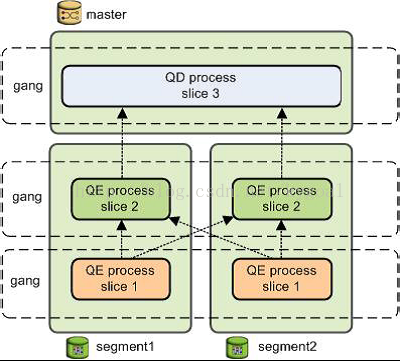
Figure 22:Query Worker Processes
24.2 关于 Pivotal查询优化器
在GPDB 4.3.5.0及更高的版本, Pivotal Query Optimizer 和 legacy query optimizer 共存。
这些章节描述了Pivotal查询优化器的功能和用法: Overview of the Pivotal Query Optimizer
• 使用 Pivotal Query Optimizer的注意事项
• Pivotal QueryOptimizer的功能和增强功能
• 改变 Pivotal Query Optimizer的行为
24.2.1 Overview of the Pivotal Query Optimizer
Pivotal Query Optimizer扩展了legacy optimizer的规划和优化能力. Pivotal Query Optimizer在多核架构中实现了更好的优化。当 Pivotal Query Optimizer启用后, GPDB会在能使用PivotalQuery Optimizer 的时候就使用它来生成查询计划
Pivotal Query Optimizer在如下几个方面增强了GPDB的查询性能优化:
• 针对分区表的查询
• 包含公用表表达式查询 (CTE)
• 包含子查询的查询
在Greenplum数据4.3.5.0及更高版本,Pivotal Query Optimizer和legacy query optimizer共存。默认情况下,GPDB使用legacy query optimizer。当Pivotal Query Optimizer 启用后,GPDB会尽可能的使用Pivotal Query Optimizer来生成查询计划。如果Pivotal Query Optimizer无法使用,那就使用legacy query optimizer。
下面显示了Pivotal Query Optimizer如何融入到查询架构中。
注意: Pivotal Query Optimizer 会忽略legacy query optimizer (planner) 的所有server 设置参数。但是,如果GPDB重新使用legacy optimizer, 则 planner server 设置参数就会影响查询计划的生成。关于legacy query optimizer (planner) server参数设置, 详见Query Tuning Parameters.
24.2.2 启用 Pivotal Query Optimizer
要启用Pivotal Query Optimizer, 你必须设置GPDB的服务器参数.
• 设置 optimizer_analyze_root_partition参数来启用分区表的根分区统计。
• 设置优化参数来启用Pivotal Query Optimizer. 你可以在如下层面设置参数:
• A specificGreenplum database
注意: 你可以通过设置optimizer_control来启用或禁用Pivotal Query Optimizer。有关服务器配置参数的信息,请参阅Greenplum数据参考指南。Greenplum DatabaseReference Guide.
重要提示:如果你要在启用Pivotal Query Optimizer的情况下在分区表上执行查询,则你必须通过执行analyze rootpartition命令来获取分区表的根分区的统计信息。analyze rootpartition只收集分区表的根分区的统计信息,而不收集叶子分区的统计信息。如果你指定了分区表的列名,则根分区和指定列的统计信息被获取。关于analyze的信息,详见Greenplum的数据库实用程序指南。Greenplum DatabaseReference Guide.
你也可以使用analyzedb来更新标的统计信息。Analyzedb可以并行更新多个表的统计信息。并且他还可以检查表的统计信息并在统计信息不及时或不存在时更新它。作为日常数据库维护的一部分,pivotal建议当分区表的叶子节点有大的数据变动时更新分区表的根分区。
24.2.2.1 设置 optimizer_analyze_root_partition参数
当 optimizer_analyze_root_partition 配置参数被设置为 on时, 当在分区表上运行analyze 命令时就会收集根分区的统计信息。Pivotal Query Optimizer 需要分区表的根分区统计信息。
1. 用gpadmin登录到GPDB的master节点。
2. 设置服务器参数,使用gpconfig来设置相应测参数为on:
$ gpconfig -c optimizer_analyze_root_partition -von 一一masteronly仅仅在master节点上
3. 重新启动数据库。 gpstop 命令会在无需关闭GPDB的情况下重新加载postgresqi.conf。
gpstop-u
24.2.2.2 Enabling the Pivotal Query Optimizer for a System
Set the server configuration parameter optimizerfor the Greenplum Database system.
1. 用gpadmin登录到GPDB的master节点。
2. 设置服务器参数,使用gpconfig来设置相应测参数为on:
$ gpconfig -c optimizer -v on --masteronly
3. 重新启动数据库。 gpstop 命令会在无需关闭GPDB的情况下重新加载postgresqi.conf。
gpstop -u
24.2.2.3 Enabling the Pivotal Query Optimizer for a Database
使用alter database 来设置单个的数据库参数。例如, 在test_db上启用 Pivotal Query Optimizer.
> ALTER DATABASE test_db SET OPTIMIZER = ON ;
24.2.2.4 Enabling the Pivotal Query Optimizer for a Session or a Query
你可以使用SET命令在一个会话中设置服务器参数。例如,你用psql连接到数据库,并用SET命令来启用Pivotal Query Optimizer:
> set optimizer = on ;
如需为特定的查询设定参数,需要在查询前执行SET命令。
24.2.3 Considerations when Using the Pivotal Query Optimizer
如需使用Pivotal Query Optimizer来执行查询,在执行查询时需要考虑。
请确保满足如下条件:
• 分区表不包含多列的分区键。
• 多层分区时统一的多层分区。详见About Uniform Multi-levelPartitioned Tables.
• 服务器参数optimizer_enable_master_only_queries被设置为on,使得只对master的系统表如pg_attribute来执行。关于这个参数的更多信息,详见Greenplum Database Reference Guide.
Note: 启用这个参数会降低短的目录查询性能。为了避免这种情况发生,仅仅在一个会话或查询时设置此参数。
分区表的根分区统计信息已获取。
如果一个分区表超过了20,000个分区,表的架构需要考虑重新设计。
Pivotal Query Optimizer会对给定的查询生成minidumps来描述优化内容。Pivotal support 使用minidump分析GPDB的相关问题。Minidump文件内容是机读格式,一般用户很难于阅读或参照其进行故障排除。这些转储文件在master的数据目录下并且以如下格式来命名:
Minidump_date_time .mdp
关于minidump的详细信息,请参阅Greenplum数据参考指南服务器配置参数optimizer_minidump。
当Pivotal Query Optimizer使用explainanalyze命令时,explain的执行计划显示有多少分区被过滤掉。被扫描的分区不予显示,为了在segment log显示那些被扫描的分区名,需要设置gp_log_dynamic_partition_pruning参数为on,命令如下:
SET gp_log_dynamic_partition_pruning = on;
24.2.4 Pivotal Query Optimizer Features and Enhancements
The Pivotal Query Optimizer包括针对特定类型的查询和操作的增强功能:
• 对分区表的查询
• 包含子查询的查询
• DML OperationEnhancements with Pivotal Query Optimizer
Pivotal Query Optimizer也包括这些优化增强:
• 改进的连接顺序
• Join-Aggregate reordering
• 排序优化
• 查询优化包含数据倾斜估计
24.2.4.1.1 针对分区表的查询
The Pivotal Query Optimizer包括以下增强功能对分区表的查询:
• 对分区的消除进行了增强.
• 支持统一多层分区表. 关于统一多层分区表, see About UniformMulti-level Partitioned Tables
• 查询计划可以包含 Partition selector operator.
• explain计划中没有把分区列举出来.
对于涉及静态分区选择那里的分区键是比较恒定的查询,Pivotal Query Optimizer在Partition Selector operator下explainoutput列出需要扫描的分区。下面的例子显示一些分区被扫描:
Partition Selector for Part_Table (dynamic scan id:1)
Filter: a > 10
Partitions selected: 1 (out of3)
对于涉及动态分区选择其中分区键相比较的变量的查询,被扫描的分区的数目将仅在查询执行是已知的。所选分区中解释输出未示出。
• 计划大小和分区数无关。
• 因分区数而导致的内存溢出错误降低了。(Out of memory errorscaused by number of partitions are reduced.)
在本例中 create table 创建一个系列的分区表。
CREATE TABLE sales(order_id int, item_id int,amount numeric(15,2),
date date, yr_qtr int)
range partitioned by yr_qtr;
Pivotal Query Optimizer 对分区表的如下类型的查询进行了优化:
• 全表扫描。分区不在计划中列出。
SELECT* FROM sales;
• 查询中包含固定的过滤,则执行分区消除。
SELECT* FROM sales WHERE yr_qtr = 201201;
• 范围选择,也执行分区消除。
SELECT * FROM sales WHERE yr_qtr BETWEEN 201301 AND201404 ;
连接中涉及分区表。在本例中,分区维表date_dim和事实表catalog_sales进行了关联
SELECT * FROM catalog_sales
WHEREdate_id IN (SELECT id FROM date_dim WHERE month=12);
24.2.4.1.2 包含子查询的查询
Pivotal Query Optimizer 对子查询更高效。子查询是嵌套在外部查询块中查询。在下面的查询中,SELECT WHERE子句中的子查询。
SELECT* FROM part
WHEREprice > (SELECTavg(price) FROM part);
Pivotal Query Optimizer也能高效的处理包含相关子查询(correlated subquery CSQ). 相关子查询是使用值从外部查询的子查询。在下面的查询,价格列在这两个外部查询和子查询中使用。
SELECT* FROM part p1
WHERE price > (SELECT avg(price) FROM part p2 WHERE p2.brand = pl.brand);
Pivotal Query Optimizer会对如下的子查询生成更高效的计划:
• CSQ in the SELECT list.
SELECT *,
(SELECT min(price) FROM part p2 WHEREp1.brand = p2.brand)
AS foo
FROMpart p1;
• CSQ in disjunctive (or)filters.
SELECTFROM part p1 WHERE p_size > 40 OR p_retailprice >
(SELECTavg(p_retailprice)
FROMpart p2
WHEREp2.p_brand = p1.p_brand)
• Nested CSQ with skip level correlations
SELECT* FROM part p1 WHERE p1.p_partkey
IN (SELECT p_partkey FROM part p2 WHEREp2.p_retailprice =
(SELECTmin(p_retailprice)
FROMpart p3
WHEREp3.p_brand = p1.p_brand)
);
Note: Nested CSQ with skip level correlations arenot supported by the legacy query optimizer.
• CSQ with aggregate and inequality. This examplecontains a CSQ with an inequality.
SELECT* FROM part p1 WHERE p1.p_retailprice =
(SELECT min(p_retailprice) FROM part p2 WHEREp2.p_brand <> p1.p_brand);
• CSQ that must return one row.
SELECTp_partkey,
(SELECTp_retailprice FROM part p2 WHERE p2.p_brand = p1.p_brand )
FROM part p1;
24.2.4.1.3 Queries that Contain CommonTable Expressions
Pivotal Query Optimizer 可以处理with字句的查询。WITH子句,也称为公用表表达式(CTE),产生存在仅用于查询临时表。这个例子查询包含一个CTE。
WITH v AS (SELECT a, sum(b) as s FROM T where c< 10 GROUP BY a)
SELECT *FROM v AS v1 , v AS v2
WHERE v1.a<> v2.a AND v1.s < v2.s;
作为查询优化的一部分,Pivotal Query Optimizer可以将谓词下推到 CTE。下面的例子, Pivotal Query Optimizer 就把等值谓词下推到CTE.
WITH v AS (SELECT a, sum(b) as s FROM T GROUP BY a)
SELECT *
FROM v as v1, v as v2, v as v3
WHERE v1.a < v2.a
AND v1.s < v3.s
AND v1.a = 10
AND v2.a = 20
AND v3.a = 30;
Pivotal Query Optimizer 可以处理如下类型的 CTE:
• CTE 定义一个或多个表。在如下查询中,CTE就定义了两个表。
WITHcte1 AS (SELECT a, sum(b) as s FROM T
where c < 10 GROUP BY a),
cte2 AS (SELECT a, s FROM cte1 where s >1000)
SELECT *
FROM cte1 as v1, cte2 as v2, cte2 as v3
WHERE v1.a < v2.a AND v1.s < v3.s;
24.2.4.1.4 DML Operation Enhancements withPivotal Query Optimizer
Pivotal Query Optimizer包含DML操作,如INSERT,UPDATE和DELETE增强。
• A DML node in a query plan is a query planoperator.
• Can appear anywhere in the plan, as a regular node(top slice only for now)
• Can have consumers
• update operations use the query plan operator Split andsupports these operations:
• update operations on the table distribution key columns.
• update operations on the table on the partition keycolumn.
This example plan shows the Split operator.
QUERY PLAN
--------------------------------------------------------------
Update (cost=0.00..5.46 rows=1 width=1)
-> Redistribute Motion 2:2(slice1; segments: 2)
Hash Key: a
-> Result (cost=0.00..3.23rows=1 width=48)
-> Split (cost=0.00..2.13 rows=1 width=40)
-> Result(cost=0.00..1.05 rows=1 width=40)
-> Table Scan on dmltest
24.2.5 Changed Behavior with the Pivotal Query Optimizer
当PivotalQuery Optimizer启用后,GPDB的数据库行为会有变化
• 允许散列键的update
• 允许update分区表的分区键值
• 支持同一分区表的查询
• 对分区表的叶子节点被更改为外部表的查询转由legacyquery optimizer来处理。
• 除了 insert, 对分区表的子表的DML操作不支持 (as of Greenplum Database 4.3.0.0).
对于insert 命令,你可以在导入数据时指定分区子表。如果指定的分区子表无效,则返回错误。不支持指定叶子子表之外的表。
• 如果create table命令中不包含distributed by,则创建的表就是随机分布。并且没有散列键或唯一键被指定。
• 非确定性的update不被支持。如下的UPDATE命令就返回一个错误。
update r set b = r.b + 1 from s where r.a in(select a from s);
• 统计数据都需要在分区表上的根表。在Analyze命令生成的根和各个分区表(叶子表)的统计数据。请参阅ANALYZE命令ROOTPARTITION条款。
• 其他节点结果在查询计划:
• Query plan Assert operator.
• Query plan Partition selector operator.
• Query plan Split operator.
• 执行explain时, Pivotal Query Optimizer生成的查询计划和legacy query optimizer不同。
• Greenplum Database adds the log file messagePlanner produced plan when the Pivotal Query Optimizer is enabled and GreenplumDatabase falls back to the legacy query optimizer to generate the query plan.
• Greenplum Database issues a warning when statisticsare missing from one or more table columns. When executing an SQL command withthe Pivotal Query Optimizer, Greenplum Database issues a warning if the commandperformance could be improved by collecting statistics on a column or set ofcolumns referenced by the command. The warning is issued on the command lineand information is added to the Greenplum Database log file. For informationabout collecting statistics on table columns, see the analyzecommand in the GreenplumDatabase Reference Guide.
24.2.6 Pivotal Query Optimizer的限制
这里是当4.3.5.0和更新版本的GPDB Pivotal Query Optimizer 启用后的限制。 Pivotal Query Optimizer 和 legacy query optimizer在 Greenplum Database 4.3.5.0 及更新版本并不能共存,因为Pivotal Query Optimizer 不支持GPDB的所有特性。
下面是特性限制
• 不支持的SQL查询功能
• 性能衰退
• GreenplumCommand Center Database Limitation
24.2.6.1 Unsupported SQL Query Features
These are unsupported features when the PivotalQuery Optimizer is enabled:
• Indexed expressions
• percentile window function
• External parameters
• These types of partitioned tables:
• Non-uniform partitioned tables.
• Partitioned tables that have been altered to use anexternal table as a leaf child partition.
• SortMergeJoin (SMJ)
• Ordered aggregations
• These analytics extensions:
• CUBE
• Multiple grouping sets
• These scalar operators:
• ROW
• ROWCOMPARE
• FIELDSELECT
• Multiple distinct qualified aggregate functions
• Inverse distribution functions
24.2.6.2 Performance Regressions
当 Pivotal Query Optimizer启用后,如下是已知的性能衰退:
• 短查询 – 对于 Pivotal Query Optimizer, 短查询可能遇到额外的开销,因为Pivotal Query Optimizer需要改进以确定最优的查询执行计划。
• analyze – 对于Pivotal Query Optimizer, analyze 命令会生成分区表的根分区的统计信息。但是对于legacy optimizer这些统计信息无需生成。
• DML operations - For Pivotal Query Optimizer, DMLenhancements including the support of updates on partition and distributionkeys might require additional overhead.
此外,增强的以前版本的特性功能,可能会导致在匹维托查询优化与执行功能的SQL语句需要额外的时间。
Greenplum Command Center Database Limitation
对于Greenplum的指挥中心监控性能,Pivotal 建议使用默认的设置 Pivotal Query Optimizer (off) for the gpperfmon ,gpperfmon 用以Greenplum Command Center. Enabling Pivotal Query Optimizer for the gpperfmondatabase is not supported. To ensure that the Pivotal Query Optimizer isdisabled for the gpperfmon database, run this command on the system where the database is installed:
ALTER DATABASE gpperfmon SET OPTIMIZER = OFF
24.2.7 Determining the Query Optimizer that is Used
当 Pivotal Query Optimizer 启用后,你可以决定是否使用Pivotal Query Optimizer 或者直接使用legacy query optimizer.
您可以检查EXPLAIN查询计划查询确定哪个查询优化是使用Greenplum数据引擎来执行查询:
• 当 Pivotal Query Optimizer 生成查询计划时, setting optimizer=on 和Pivotal Query Optimizer 版本在查询计划的最后面会显示出来. 例如.
Settings: optimizer=on
Optimizer status: PQO version 1.584
如果GPDB使用legacy optimizer 来生成查询计划, setting optimizer=on 和 legacy query optimizer 会显示在查询计划的最后面。例如:
Settings: optimizer=on
Optimizer status: legacy query optimizer
当服务器的参数OPTIMIZER 被关闭时, 会在查询计划的末尾显示如下信息:
Settings: optimizer=off
Optimizer status: legacy query optimizer[1]
24.2.7.1 Examples
这个例子显示了启用了Pivotal Query Optimizer时,针对分区表运行查询的差异。
This create tablestatement creates a table with single level partitions:
CREATE TABLE sales (trans_id int, date date,
amountdecimal(9,2), region text)
DISTRIBUTEDBY (trans_id)
PARTITIONBY RANGE (date)
(START(date '20110101')
INCLUSIVE END (date '20120101')
EXCLUSIVE EVERY (INTERVAL '1 month'),
DEFAULT PARTITION outlying_dates );
如下查询被Pivotal Query Optimizer 支持并且不会生成查询错误:
select* from sales ;
The explain planoutput lists only the number of selected partitions.
-> Partition Selector for sales (dynamic scanid: 1) (cost=10.00..100.00rows=50
width=4)
Partitions selected: 13(out of 13)
如果对分区表的查询不被Pivotal Query Optimizer支持,则GPDB使用legacy optimizer. 由egacyoptimizer生成的查询计划列出了被选择的分区。在下例中,显示了一个查询计划的部分被选中的分区。
-> Append (cost=0.00..0.00 rows=26 width=53)
-> Seq Scan on sales2 1 prt 7 2 prt usa sales2 (cost=0.00..0.00 rows=1width=53)
-> Seq Scan on sales2 1 prt 7 2 prt asia sales2(cost=0.00..0.00 rows=1 width=53) _
这个例子说明,GPDB从Pivotal Query Optimizer 落回到legacy query optimizer。
当如下查询执行时,GPDB落回到legacy query optimizer.
explainselect * from pg_class;
并且一个显示一个附加的消息。这个附加消息包含为什么Pivotal Query Optimizer没有执行这个查询的原因。
NOTICE,"Feature not supported by the Pivotal Query Optimizer: Queries onmaster-only tables"
24.2.8 About Uniform Multi-levelPartitioned Tables
Pivotal Query Optimizer supports queries on amulti-level partitioned (MLP) table if the MLP table is a uniform partitioned table. A multi-level partitioned table is a partitioned table that was createdwith the subpartition clause. A uniform partitioned table must meet these requirements.
• Thepartitioned table structure is uniform. Each partition node at the same levelmust have the same hierarchical structure.
• The partition key constraints must be consistentand uniform. At each subpartition level, the sets of constraints on the childtables created for each branch must match.
You can display information about partitionedtables in several ways, including displaying information from these sources:
• The pg_partitions system view containsinformation on the structure of a partitioned table.
• The pg_constraint system catalogtable contains information on table constraints.
• The psql meta command \d+ tablenamedisplays the table constraints for child leaf tables of a partitioned table.
24.2.8.1 Example
This create table command creates a uniform partitioned table.
CREATE TABLE mlp (id int, year int, month int, day int,
region text)
DISTRIBUTED BY (id)
PARTITION BY RANGE ( year)
SUBPARTITION BY LIST (region)
SUBPARTITION TEMPLATE (
SUBPARTITION usa VALUES ( 'usa'),
SUBPARTITION europe VALUES ('europe'),
SUBPARTITION asia VALUES ('asia'))
( START ( 2000) END ( 2010) EVERY ( 5));
These are child tables and the partition hierarchythat are created for the table mlp. This hierarchy consists of one subpartitionlevel that contains two branches.
mlp_1_prt_11
mlp_1_prt_11_2_prt_usa
mlp_1_prt_11_2_prt_europe
mlp_1_prt_11_2_prt_asia
mlp_1_prt_21
mlp_1_prt_21_2_prt_usa
mlp_1_prt_21_2_prt_europe
mlp_1_prt_21_2_prt_asia
表中的层次结构是均匀的,每个分区包含一组三个子表(子分区)。该区域的子分区的约束是均匀的,该组上的分支表mlp_1_prt_11子表的约束是相同的上跳转表的子表的约束mlp_1_prt_21.
As a quick check, this query displays theconstraints for the partitions.
WITH tbl AS (SELECT oid, partitionlevel AS level,
partitiontablename AS part
FROM pg_partitions, pg_class
WHERE tablename = 'mlp' ANDpartitiontablename=relname
AND partitionlevel=1 )
SELECT tbl.part, consrc
FROM tbl, pg_constraint
WHEREtbl.oid = conrelid ORDER BY consrc;
Note: You will need modify the query for morecomplex partitioned tables. 例如, the query does not account for table names indifferent schemas.
The consrc column displays constraints on thesubpartitions. The set of region constraints for the subpartitions in mlp_1_prt_1 match the constraintsfor the subpartitions in mlp_1_prt_2. The constraints foryear are inherited from the parent branch tables.
part | consrc
---------------------------------+------------------------------------
mlp_1_prt_2_2_prt_asia | (region ='asia'::text)
mlp_1_prt_1_2_prt_asia | (region ='asia'::text)
mlp_1_prt_2_2_prt_europe | (region ='europe'::text)
mlp_1_prt_1_2_prt_europe | (region ='europe'::text)
mlp_1_prt_1_2_prt_usa | (region ='usa'::text)
mlp_1_prt_2_2_prt_usa | (region ='usa'::text)
mlp_1_prt_1_2_prt_asia | ((year>= 2000) AND (year < 2005))
mlp_1_prt_1_2_prt_usa | ((year>= 2000) AND (year < 2005))
mlp_1_prt_1_2_prt_europe | ((year>= 2000) AND (year < 2005))
mlp_1_prt_2_2_prt_usa | ((year>= 2005) AND (year < 2010))
mlp_1_prt_2_2_prt_asia | ((year>= 2005) AND (year < 2010))
mlp_1_prt_2_2_prt_europe | ((year>= 2005) AND (year < 2010))
(12 rows)
如果添加一个默认的分区来使用这个命令的例子分区表:
ALTERTABLE mlp ADD DEFAULT PARTITION def
分区表保持一个统一的分区表。默认分区创建的分支包含三个子表和子表匹配的子表的约束现有的套组约束。
在上面的例子中,如果删除该子分区mlp_1_prt_21_2_prt_asia并添加另一子分区的区域加拿大,约束不再是均匀的。
ALTERTABLE mlp ALTER PARTITION FOR (RANK(2))
DROPPARTITION asia ;
ALTERTABLE mlp ALTER PARTITION FOR (RANK(2))
ADDPARTITION canada VALUES ('canada');
另外,如果你mlp_1_prt_21下添加一个分区加拿大,划分层次不统一。
但是,如果你添加加拿大子分区既mlp_1_prt_21和mlp_1_prt_11了原来的分区表的,它仍然是一个统一的分区表。
注意:只有在在划分级别的集合分区的限制必须是相同的。分区的名称可以是不同的。
24.3 定义查询
Greenplum的数据库是基于PostgreSQL的执行SQL标准。
本主题介绍了如何构建在Greenplum数据的SQL查询。
• SQL词典
• SQL 值表达式
24.3.1 SQL词典
SQL是用于访问数据库的标准语言。语言包括,使数据的存储,检索,分析,观看,操纵等元素。你可以使用GPDB可解析的SQL来操纵数据库。SQL查询包括一个命令序列。命令包括在正确的语法为了有效的标记,以分号结束序列的(;)。
有关SQL命令的详细信息,请参阅Greenplum数据参考指南。
Greenplum的数据库使用PostgreSQL的结构和语法,有一些例外。有关SQL规则和概念在PostgreSQL的更多信息,请参见“SQL语法”PostgreSQL的文档中获得。
24.3.2 SQL Value Expressions
SQL值表达式由一个或多个值,符号,运算,SQL函数和数据。表达式比较数据或执行计算并返回一个值作为结果。计算包括逻辑,算术和设置操作。
如下是值表达式:
• An aggregate expression
• An array constructor
• A column reference
• A constant or literal value
• A correlated subquery
• A field selection expression
• A function call
• A new column value in an insert or update
• An operator invocation column reference
• A positional parameter reference, in the body of afunction definition or prepared statement
• A row constructor
• A scalar subquery
• A search condition in a whereclause
• A target list of a select command
• A type cast
• A value expression in parentheses, useful to groupsub-expressions and override precedence
• A window expression
SQL构造,如函数和操作符表达式,但不遵循任何通用的语法规则。有关这些结构的更多信息,请参阅使用函数和操作符。Using Functions and Operators.
24.3.2.1 Column References
A column reference has the form:
correlation.columnname
在这里,相关性是一个表名(可能有模式名修饰)或用FROM子句或关键字之一新旧定义的表的别名。 NEW和OLD只能出现在重写规则,但你可以在任何SQL语句中使用其他相关的名字。如果列名在所有表中的唯一的查询,可以省略“相关性”。列引用的一部分。
24.3.2.2 Positional Parameters
位置参数的参数,你通过它们的位置在一系列的参数参考SQL语句或功能。例如,$ 1指第一个参数,$ 2指第二个参数,依此类推。位置参数的值是从外部的SQL语句,或者当被调用SQL函数提供的参数设置。一些客户端库支持从SQL命令,在这种情况下,参数指出的行中的数据值分别指定的数据值。一个参数引用的形式为:
$number
例如:
CREATE FUNCTION dept(text) RETURNS dept
AS $$ SELECT * FROM dept WHERE name= $1 $$
LANGUAGESQL;
Here, the $1 references the value ofthe first function argument whenever the function is invoked.
24.3.2.3 下标
如果一个表达式生成一个数组类型的值,可以按如下方式提取数组值的特定元素:
expression[subscript]
可以提取多个相邻的元件,称为阵列片,如下(包括括号):
expression[lower_subscript:upper_subscript]
每个下标是一个表达和产生一个整数值。
数组表达式通常必须在括号,但你可以省略括号时要下标表达式是列引用或位置参数。您可以连接多个标时,原来的数组是多维的。例如(包括括号内):
mytable.arraycolumn[4]
mytable.two_d_column[17][34]
$1[10:42]
(arrayfunction(a,b))[42]
24.3.2.4 Field Selection
如果一个表达式生成一个复合类型(行类型)的值,可以按如下方式提取行的具体领域:
expression. fieldname
行表达,通常必须在括号,但是,当要选择的表达从是一个表参照或位置参数,可以省略这些括号。例如:
mytable.mycolumn
$1.somecolumn
(rowfunction(a,b)).col3
限定的列引用是字段选择语法的特例。
24.3.2.5 操作符的调用
操作调用有以下可能的语法:
expression operator expression(binary infixoperator) operator expression(unary prefixoperator) expression operator(unarypostfix operator)
Where operator is an operator token, one of the key words and, or, or not, orqualified operator name in the form:
OPERATOR(schema.operatorname)
可用的运营商和他们是否是一元或二元取决于系统或用户定义的运算符。有关内置运营商的更多信息,请参阅内置函数和操作符。Built-in Functions and Operators.
24.3.2.6 函数调用
函数调用的语法是一个函数(可能有模式名修饰),后面用括号括起来的参数列表的名称:
function ([expression [, expression ...]])
例如, the following function call computes the square root of 2:
sqrt(2)
See the Greenplum Database Reference Guide for lists of the built-in functions by category. You can add customfunctions, too.
24.3.2.7 Aggregate Expressions
一个聚集表达式跨查询选择行应用聚合函数。聚合函数上执行的一组值的计算,并返回一个值,如设定值的总和或平均。聚集表达式的语法是下列之一:
• aggregate_name( expression[ , ... ] ) — operatesacross all input rows for which the expected result value is non-null. all is the default.
• eggregate_name(all expression [ , ... ]) — operates identically to the first form because all is the default.
• aggregate_name(DISTINCT expression [ , ... ] ) —operates across all distinct non-null values of input rows.
• aggregate_name(*) — operates on all rows withvalues both null and non-null. Generally, this form is most useful for thecount(*) aggregate function.
这里aggregate_name是前面定义的聚集(可能有模式修饰)和表达任何值表达式不包含聚集表达式。
例如, count(*) yields the total number of input rows, count(fi)yields the number of input rows in which fi is non-null, and count(distinct fi) yields the number of distinctnon-null values of fi.
对于预定义的聚合函数,请参阅内置函数和操作符。您还可以添加自定义聚合函数。
Greenplum的数据库提供的中间聚合函数,它返回PERCENTILE_CONT结果和逆分布函数的特殊聚合表达式如下五十百分位:
PERCENTILE_CONT(_percentage_)WITHIN GROUP (ORDER BY _expression_) PERCENTILE_DISC(_percentage_) WITHIN GROUP(ORDER BY _expression_)
Currently you can useonly these two expressions with the keyword within group.
24.3.2.7.1 Limitations of AggregateExpressions
The following are current limitations of theaggregate expressions:
• Greenplum的数据库不支持以下关键字:ALL,DISTINCT, FILTER and OVER. SeeTable 50: AdvancedAggregate Functions for more details.
• 一个聚集表达式只能出现在结果列表或者具有SELECT命令的子句。一个聚集表达式只能出现在结果列表或者具有SELECT命令的子句。
禁止在其他语法,如WHERE,因为这些语法都聚集形式的结果前,在逻辑上进行评估。此限制适用于该聚集所属的查询级别。
• 当集合表达式出现在一个子查询,聚集通常是在子查询的行评估。如果聚集的参数仅包含外级变量,聚合属于最近这类外水平和评估在该查询中的行。集合表达式作为一个整体,然后在它出现的子查询的外部参考,聚合表达式作为一个恒定的子查询中的任何一个评价。 SeeScalarSubqueries and Table 47: Built-in functions and operators.
• Greenplum的数据库不支持包含多个输入表达式的DISTINCT。
24.3.2.8 Window Expressions
窗口表达式允许应用程序开发者更容易编写使用标准的SQL命令复杂的在线分析处理(OLAP)查询。例如,使用窗口表达式,用户可以计算移动平均数额或在不同的时间间隔,重新聚合和行列选定的列值发生改变,并表达简单来说复杂的比率。
一个窗口表达式表示施加到一个窗框,这是在一个特殊的OVER()子句定义的窗函数的应用程序。窗口分区是一组行组合在一起应用窗口的功能。不同于聚合函数,它为每个行组返回一个结果值,窗口函数返回一个结果值的每一行,但该值与在一个特定的窗口分区对于行计算。如果没有指定分区,窗口函数计算在整个中间结果集。
窗口表达式的语法是:
window_function ( [expression [, ...]] ) OVER (window_specification )
其中,窗函数是在表48中列出的功能之一:窗口功能,表现为任何不包含一个窗口的表达,和窗口规范值表达为:
[window_name]
[PARTITION BY expression [, ...]]
[[ORDER BY expression [ASC | DESC | USING operator] [, ...]
[{RANGE | ROWS}
{ UNBOUNDED PRECEDING
| expression PRECEDING
| CURRENT ROW
| BETWEEN window_frame_bound ANDwindow_frame_bound }]]
and where window—frame—bound can be one of:
UNBOUNDEDPRECEDING
expressionPRECEDING
CURRENTROW
expressionFOLLOWING
UNBOUNDEDFOLLOWING
一个窗口表达式只能在SELECT命令的选择列表中。例如:
SELECTcount(*) OVER(PARTITION BY customer_id), * FROM sales;
OVER子句从其他聚合或报告功能区分窗口功能。 OVER子句定义要施加的窗口函数的窗口规范。窗口规范具有以下特点:
• PARTITION BY子句定义要施加的窗口函数的窗口分区。如果省略,整个结果集被视为一个分区。The partition by clause defines the window partitions to which the window function isapplied. If omitted, the entire result set is treated as one partition.
• ORDER BY子句定义窗口分区内部数据的排序定义。窗口函数的ORDER BY 子句和普通的ORDER BY 有很大的不同。窗口函数需要ORDER BY 子句来进行排名,因此需要明确需要排名的度量值。对于OLAP聚合,ORDER BY 子句需要在窗体使用 (the ROWS | RANGE clause).
注:数据类型的列没有一个连贯的排序,如时间,不是ORDER BY子句的比较好的候选列。Time, with or without a specified time zone,缺乏连贯排序,因为对其加减没有产生预期的效果。例如, the following is not generally true: x::time < x::time + '2 hour'::interval
• rows/range 子句定义汇总(非排名)窗口功能的窗框。窗框定义窗口分区中的一组行。当定义一个窗框,窗函数计算在此移动框架中的内容,而不是整个窗口分区的固定内容。 Window frames are row-based (ROWS) or value-based (RANGE).
24.3.2.9 Type Casts
一个类型转换声明一个从一种数据类型到另一种转换。 Greenplum的数据库接受两个相当的语法为类型转换:
CAST ( expression AS type ) expression::type
cast语法遵从SQL; ::语法是从PostgreSQL用法继承过来的。
适用于已知类型的值表达式强制转换为一个运行时类型转换。转换成功只有一个合适的类型转换函数的定义。这不同于使用常量的转换。适用于字符串文本的转换表示一个类型为常量值的初始分配,所以它成功的任何类型的,如果字符串的内容是为数据类型的输入语法接受。
通常你可以省略明确的类型转换,如果没有关于值表达式必须产生歧义的类型;例如,当它被分配到一个表列,系统将自动应用类型转换。
系统仅在系统目录里标记为"OK to apply implicitly" 的项才执行自动转换。其他的转换必须明确的声明转换语法,以防止在用户不知情的情况下执行意外的转换。
24.3.2.10 Scalar Subqueries
标量子查询是在括号中的SELECT查询只返回单行单列。不要将返回多行或多列的查询作为scalar subquery。这个查询执行后返回的结果被使用在其附近的表达式中。一个相关标量子查询包含了对外部查询块引用。A correlated scalar subquery contains references to the outer query block.
24.3.2.11 Correlated Subqueries
相关子查询(CSQ)是一个包含WHERE语法或目标列包含对parent outer引用的查询。CSQ的高效表达的另一个查询结果方面的成果。Greenplum的数据库支持相关子查询提供与现有的许多应用程序的兼容性。一个CSQ是一个标量或表子查询,取决于它是否返回一个或多个行。 Greenplum的数据库不支持跳过级相关相关子查询。
A correlated subquery (CSQ) is a SELECT query witha WHERE clause or target list that contains references to the parent outerclause. CSQs efficiently express results in terms of results of another query.Greenplum Database supports correlated subqueries that provide compatibilitywith many existing applications. A CSQ is a scalar or table subquery, dependingon whether it returns one or multiple rows. Greenplum Database does not supportcorrelated subqueries with skip-level correlations.
24.3.2.12 Correlated Subquery Examples
24.3.2.12.1 Example 1 - Scalar correlatedsubquery
SELECT * FROMt1 WHERE t1.x
> (SELECT MAX(t2.x) FROM t2 WHERE t2.y =t1.y);
24.3.2.12.2 Example 2- Correlated EXISTSsubquery
SELECT * FROM t1 WHERE
EXISTS (SELECT 1 FROM t2 WHERE t2.x = t1.x);
Greenplum Database uses one of the followingmethods to run CSQs:
• Unnest the CSQ into join operations UNNEST CSQ的进入连接操作 – 这种方法最有效, 这也是Greenplum Database 如何执行大多数的CSQs, 包括来自TPC-H基准的查询。
• 在外部查询的每一行运行CSQ -这种方法比较低效, 这就是Greenplum Database执行在select列表中包含CSQs in 或者包含OR条件连接的查询。
以下实例说明如何改写一些这些类型的查询,以提高性能。
24.3.2.12.3 Example 3 - CSQ in the SelectList
原始查询
SELECT T1.a,
(SELECT COUNT(DISTINCT T2.z)FROM t2 WHERE t1.x = t2.y) dt2
FROM t1;
重写此查询执行与T1内部联接,然后再执行左键再次加入与T1。重写适用于只等值加入的相关条件。
Rewrite this query to perform an inner join with t1 first and then perform aleft join with t1 again. The rewrite applies for only an equijoin inthe correlated condition.
Rewritten Query
SELECT t1.a, dt2 FROM t1
LEFT JOIN
(SELECT t2.y AS csq_y, COUNT(DISTINCTt2.z) AS dt2
FROM t1, t2 WHERE t1.x = t2.y
GROUP BY t1.x)
ON (t1.x = csq_y);
24.3.2.12.4 Example 4 - CSQs connected byOR Clauses
Original Query
SELECT * FROM t1
WHERE
x > (SELECT COUNT(*) FROM t2 WHERE t1.x =t2.x)
OR x< (SELECT COUNT(*) FROM t3 WHERE t1.y = t3.y)
Rewrite this query to separate it into two partswith a union on the or conditions.
Rewritten Query
SELECT * FROM t1
WHERE x > (SELECT count(*)FROM t2 WHERE t1.x = t2.x)
UNION
SELECT * FROM t1
WHEREx < (SELECT count(*) FROM t3 WHERE t1.y = t3.y)
To view the query plan, use explain select or explain analyze select. Subplan nodes in the query plan indicate that the query will run on everyrow of the outer query, and the query is a candidate for rewriting. For moreinformation about these statements, seeQuery Profiling.
24.3.2.13 Advanced Table Functions
Greenplum的数据库支持表函数与表值表达式。您可以使用ORDER BY子句高级表函数的输入行进行排序。可以用分散BY子句重新分配它们,以指定一个或多个列或其中具有指定特征的行提供给相同的处理的表达式。这种用法类似于使用创建表时分布式BY子句,但在查询运行时出现的重新分配。
下面的命令使用与散射表函数由该GPText功能gptext.index)条款(来用消息表数据的索引mytest.articles:
SELECT * FROM gptext.index(TABLE(SELECT * FROM messages
SCATTER BY distrib_id), 'mytest.articles');
Note:
根据数据的分布,Greenplum数据引擎自动并行表函数与在群集的节点表值参数。
有关功能gptext.index()的信息,请参阅Pivotal GPText文档。
24.3.2.14 Array Constructors
数组构造函数是建立在价值为它的成员元素的数组值的表达式。一个简单的数组构造由关键字ARRAY,一个左方括号中[用逗号为数组元素值分隔的一个或多个表达式和一个右括号。例如,
SELECTARRAY[1,2,3+4]; array
{1,2,7}
数组元素类型是其成员表达式的常见类型,使用同样的规则,作为UNION或CASE构造决定的。
你可以建立由嵌套数组构造多维数组值。在内部构造,则可以省略关键字ARRAY。例如,下面的两个SELECT语句产生相同的结果:
SELECT ARRAY[ARRAY[1,2], ARRAY[3,4]];
SELECT ARRAY[[1,2],[3,4]];
array
---------------
{{1,2},{3,4}}
因为多维数组必须为矩形,在同一级别内的构造必须产生相同尺寸的子阵列。
多维数组构造元件不限于一个子阵列构建体;它们是什么,产生适当的一种阵列。例如:
CREATE TABLE arr(f1 int[], f2 int[]);
INSERT INTO arr VALUES (ARRAY[[1,2],[3,4]],
ARRAY[[5,6],[7,8]]);
SELECT ARRAY[f1, f2, '{{9,10},{11,12}}'::int[]] FROM arr;
array
------------------------------------------------
{{{1,2},{3,4}},{{5,6},{7,8}},{{9,10},{11,12}}}
您可以构建从子查询的结果数组。写用关键字ARRAY后面括号中的子查询数组构造。例如:
SELECT ARRAY(SELECT oid FROM pg_proc WHERE proname LIKE 'bytea%');
?column?
-----------------------------------------------------------
{2011,1954,1948,1952,1951,1244,1950,2005,1949,1953,2006,31}
子查询必须返回单列。由此产生的一维数组有子查询结果的每一行的元素,匹配的子查询的输出列的元素类型。与ARRAY建立的数组值的脚标总是从1开始。
24.3.2.15 Row Constructors
行构造函数是建立从值其成员字段行值(也称为复合值)的表达式。例如,
SELECT ROW(1,2.5,'this is a test');
行构造有语法rowvalue.*,它扩展到该行的值的元素的列表,当您使用的语法。*在SELECT列表的顶部水平。例如,如果表T有列f1和F2,以下查询是相同的:
SELECT ROW(t.*, 42) FROM t;
SELECT ROW(t.f1, t.f2, 42) FROM t;
默认情况下,由行式所创造的价值有一个匿名的记录类型。如果有必要,它可以转换为一个名为复合类型 - 无论是表的行类型,或者用CREATE TYPE AS创建的复合类型。为了避免歧义,可以明确,如果有必要投的价值。例如:
CREATE TABLE mytable(f1 int, f2 float, f3 text);
CREATE FUNCTION getf1(mytable) RETURNS int AS 'SELECT $1.f1'
LANGUAGE SQL;
在下面的查询中,你不需要映射值,因为只有一个getf1()函数,因此不会产生歧义:
SELECT getf1(ROW(1,2.5,'this is a test'));
getf1
-------
1
CREATE TYPE myrowtype AS (f1 int, f2 text, f3 numeric);
CREATE FUNCTION getf1(myrowtype) RETURNS int AS 'SELECT
$1.f1' LANGUAGE SQL;
现在我们需要一个投以表明调用哪个函数:
SELECT getf1(ROW(1,2.5,'this is atest'));
ERROR: function getf1(record) isnot unique
SELECT getf1(ROW(1,2.5,'this is atest')::mytable);
getf1
-------
1
SELECT getf1(CAST(ROW(11,'this isa test',2.5) AS
myrowtype));
getf1
-------
11
可以使用行构造来构建要被存储在一个复合型的表列的复合值或将被传递到一个接受复合参数的功能。
24.3.2.16 Expression Evaluation Rules
子表达式的计算顺序是不确定的。操作者或功能的输入不一定评估左到右或任何其它固定的顺序。
如果可以通过评估仅表达的某些部分确定的表达式的结果,则其他子表达式可能不会在所有评估。例如,在下面的表达式:
SELECT true OR somefunc();
Somefunc() 可能不会在所有被调用。同样如此在以下表达式:
SELECTsomefunc() OR true;
在一些运营商的编程语言中boolean操作符不一定是从左到右的执行顺序。
不要使用带有副作用的函数作为复杂表达式的一部分,特别是在where和HAVING子句,因为开发一个执行计划时,这些字句被广泛地重新处理。在这些条款布尔表达式(AND/ OR / NOT的组合),可以在布尔代数法律允许的任何方式进行重组。
使用CASE构造来强制计算顺序。下面的例子是为了避免被零除在WHERE子句中的不值得信任的方式:
SELECT ... WHERE x <> 0 AND y/x > 1.5;
下面的例子显示了一个可信赖的计算顺序:
SELECT ... WHERE CASE WHEN x <> 0 THEN y/x > 1.5 ELSE false
END;
这种情况下,构造失败使用优化的尝试;仅在必要时才使用它。
This case construct usage defeats optimization attempts; useit only when necessary.
24.4 Using Functions and Operators
Greenplum Database evaluates functions andoperators used in SQL expressions. Some functions and operators are onlyallowed to execute on the master since they could lead to inconsistencies insegment databases.
• UsingFunctions in Greenplum Database
• Built-inFunctions and Operators
24.4.1 Using Functions in Greenplum Database
Table 46: Functions in Greenplum Database
| Function Type | Greenplum Support | Description | Comments |
| IMMUTABLE | Yes | Relies only on information directly in its argument list. Given the same argument values, always returns the same result. 仅依赖于直接在它的参数列表信息。 给同样的参数值,总是返回相同的结果。 |
|
| STABLE | Yes, in most cases | Within a single table scan, returns the same result for same argument values, but results change across SQL statements. 在单个表扫描,对某些输入参数返回相同的参数值相同的结果,但结果改变整个SQL语句。 | Results depend on database lookups or parameter values. current timestamp family of functions is stable; values do not change within an execution. 结果取决于数据库查询或参数值。 current timestamp的功能是STABLE;在一次执行内值不变。 |
| VOLATILE | Restricted | Function values can change within a single table scan. 例如: random() , currval(), timeofday(). | Any function with side effects is volatile, even if its result is predictable. 例如: setval(). |
在Greenplum的数据库中,数据被划分跨段 - 每段是一种独特的PostgreSQL数据库。为了防止不一致或意外的结果,不允许在段级别执行标记为可变的SQL命令,或者更改数据库。例如,函数,如setvai()不允许在Greenplum数据分布式数据执行,因为它们可能会导致段实例之间的数据不一致。
为了确保数据的一致性,你可以放心地在master执行VOLATILE 和 STABLE的函数来评估和执行。例如,下面的语句在master上运行(不带FROM子句的语句):
SELECT setval('myseq', 201);
SELECT foo();
如果语句有包含分布表,并在FROM子句功能的FROM子句返回一组行,该语句可以在运行段:
SELECT * from foo();
Greenplum Database does not support functions thatreturn a table reference (rangeFuncs) or functions that use the refcursordatatype. Greenplum的数据库不支持返回表引用(范围功能)或使用refcursor数据类型的函数功能。
24.4.2 User-Defined Functions
Greenplum的数据库支持用户自定义的功能。请参阅Extending SQL文档在SQL中获取更多信息。.
用CREATE FUNCTION语句来注册作为在Greenplum数据引擎使用函数描述使用用户定义的函数。默认情况下,用户定义的函数声明为volatile, 所以如果你的用户定义的函数是不变或稳定,则必须指定在您注册的功能正确的volatility 层级。
当您创建用户定义的函数,避免使用致命错误或破坏性的调用。Greenplum的数据库可能会以这样的错误响应以突然关机或重启。
在Greenplum数据引擎,用户创建的函数的共享库文件必须驻留在Greenplum数据阵列上每个主机 (masters, segments, and mirrors)的相同的库路径。
24.4.3 Built-in Functions and Operators
下表列出了PostgreSQL支持的内置函数和运算符的类别。所有的功能和运营商都在Greenplum数据作为支持PostgreSQL中具有稳定的和不稳定的功能,这是受在Greenplum数据引擎使用功能限制规定的除外。请参阅PostgreSQL文档的功能和操作部分,了解这些内置的函数和运算符的更多信息。 Functions and Operators s
Table 47: Built-in functions and operators
| Operator/Function Category | VOLATILE Functions | STABLE Functions | Restrictions |
|
|
|
| |
|
|
|
| |
| random setseed |
|
| |
| All built-in conversion functions | convert pg_client_encoding |
| |
|
|
|
| |
|
|
|
| |
|
|
|
| |
|
| to_char to_timestamp |
| |
| Operator/Function Category | VOLATILE Functions | STABLE Functions | Restrictions |
| timeofday | age current_date current_time current_timestamp localtime localtimestamp now |
| |
|
|
|
| |
|
|
|
| |
| currval lastval nextval setval |
|
| |
|
|
|
| |
|
| All array functions |
| |
|
|
|
| |
|
|
|
| |
|
|
|
| |
| generate_series |
|
| |
|
| All session information functions All access privilege inquiry functions All schema visibility inquiry functions All system catalog information functions All comment information functions |
| |
| Operator/Function Category | VOLATILE Functions | STABLE Functions | Restrictions |
| set_config pg_cancel_backend pg_reload_conf pg_rotate_logfile pg_start_backup pg_stop_backup pg_size_pretty pg_ls_dir pg_read_file pg_stat_file | current_setting All database object size functions | Note: The function pg column size displays bytes required to store the value, perhaps with TOAST compression. | |
|
| xmlagg(xml) xmlexists(text, xml) xml_is_well_formed(text) xml_is_well_formed_ document(text) xml_is_well_formed_ content(text) xpath(text, xml) xpath(text, xml, text[]) xpath_exists(text, xml) xpath_exists(text, xml, text[]) xml(text) text(xml) xmlcomment(xml) xmlconcat2(xml, xml) |
|
24.4.4 Window Functions
The following built-in window functions areGreenplum extensions to the PostgreSQL database. All window functions are immutable. Formore information about window functions, seeWindow Expressions.
| Function | Return Type | Full Syntax | Description |
| cume dist() | double precision | CUME DIST() OVER ( [PARTITION BY expr ] order by expr ) | Calculates the cumulative distribution of a value in a group of values. Rows with equal values always evaluate to the same cumulative distribution value. 计算值的一组值中的累积分布。用相等值的行始终计算相同的累积分布值。 |
| dense rank() | bigint | DENSE RANK () OVER ( [PARTITION BY expr ] ORDER BY expr ) | Computes the rank of a row in an ordered group of rows without skipping rank values. Rows with equal values are given the same rank value. 在计算一组有序行的行的排名而不跳过等级值。用相等值的行被赋予相同的排名值。 |
| first value( expr) | same as input expr type | FIRSTVALUE( expr ) OVER ([PARTITION BY expr] ORDER BY expr [rows|range frame_expr ]) | Returns the first value in an ordered set of values. 返回有序组值中的第一值。 |
| lag(expr [,offset] [,default]) | same as input expr type | lag( expr [, offset ] [, default ]) OVER ( [PARTITION BY expr ] ORDER BY expr ) | Provides access to more than one row of the same table without doing a self join. Given a series of rows returned from a query and a position of the cursor, lag provides access to a row at a given physical offset prior to that position. The default offset is 1. default sets the value that is returned if the offset goes beyond the scope of the window. If default is not specified, the default value is null. 提供对同一个表的多个行而不做自连接。鉴于一系列从查询返回的行和光标的位置,LAG提供了在给定的物理到该位置之前的偏移访问一行。缺省偏移量是1。默认集,如果所述偏移超出窗的范围时返回的值。如果未指定默认值,则默认值为null。 |
| last valueexpr | same as input expr type | LAST VALUE( expr) OVER ([PARTITION BY expr] ORDER BY expr [ROWS|RANGE ) | Returns the last value in an ordered set of values. |
| Function | Return Type | Full Syntax | Description |
| lead(expr [,offset] [,default]) | same as input expr type | LEAD( expr [, offset] [,xppddefailt]) OVER ( [PARTITION BYexpr] ORDER BY expr ) | Provides access to more than one row of the same table without doing a self join. Given a series of rows returned from a query and a position of the cursor, lead provides access to a row at a given physical offset after that position. If offset is not specified, the default offset is 1. default sets the value that is returned if the offset goes beyond the scope of the window. If default is not specified, the default value is null. 提供对同一个表的多个行而不做自连接。定的一系列从查询返回的行和所述光标的位置,引线提供在给定的物理该位置之后的偏移存取的行。 如果偏移量未指定,则缺省偏移量是1。默认集,如果所述偏移超出窗的范围时返回的值。如果未指定默认值,则默认值为null。 |
| ntile(expr) | bigint | NTILE(expr) OVER ( [PARTITION BY expr] ORDER BY expr ) | Divides an ordered data set into a number of buckets (as defined by expr) and assigns a bucket number to each row. |
| percent rank() | double precision | PERCENT RANK () OVER ( [PARTITION BY expr] ORDER BY expr ) | Calculates the rank of a hypothetical row R minus 1, divided by 1 less than the number of rows being evaluated (within a window partition). |
| rank() | bigint | RANK () OVER ( [PARTITION BY expr] ORDER BY expr ) | Calculates the rank of a row in an ordered group of values. Rows with equal values for the ranking criteria receive the same rank. The number of tied rows are added to the rank number to calculate the next rank value. Ranks may not be consecutive numbers in this case. |
| row number() | bigint | ROW NUMBER () OVER ( [PARTITION BY expr] ORDER BY expr ) | Assigns a unique number to each row to which it is applied (either each row in a window partition or each row of the query). |
24.4.5 高级分析函数
The following built-in advanced analytic functionsare Greenplum extensions of the PostgreSQL database. Analytic functions are immutable.
Table 49: Advanced Analytic Functions
| Function | Return Type | Full Syntax | Description |
| matrix add(array[], array[]) | smallint[], int[], bigint[], float[] | matrix add( array[[1,1], [2,2]], array[[3,4], [5,6]]) | Adds two twodimensional matrices. The matrices must be conformable. 再添两个二维矩阵。矩阵必须兼容。 |
| matrix multiply( array[], array[]) | smallint[]int[], bigint[], float[] | matrix multiply( array[[2,0, [0,2,0],[0,0,2]], array[[3,0,3], [0,3,0],[0,0,3]]) | Multiplies two, three-dimensional arrays. The matrices must be conformable. 将两个,三维阵列。矩阵必须兼容。 |
| matrix multiply( array[], expr) | int[], float[] | matrix multiply( array[[1,1, [2,2,2], [3,3,3]], 2) | Multiplies a two-dimensional array and a scalar numeric value. 二维阵列和一个标量数值相乘。 |
| matrix transpose( array[]) | Same as input array type. | matrix transpose( array [[1,1,1],[2,2,2]]) | Transposes a twodimensional array. 调换一个二维阵列。 |
| pinv(array []) | smallint[]int[], bigint[], float[] | pinv(array[[2. 5,0,0],[0,1,0], [0,0,.5]]) | Calculates the Moore- Penrose pseudoinverse of a matrix. 计算矩阵的穆尔 - 彭罗斯伪逆。 |
| unnest (array[]) | set of anyelement | unnest( array['one', 'row', 'per', 'item']) | Transforms a one dimensional array into rows. Returns a set of anyelement, a polymorphic pseud^type in PostgreSQL. |
Table 50: Advanced Aggregate Functions
| Function | Return Type | Full Syntax | Description |
| MEDIAN (expr) | timestamp, | MEDIAN (expression) | Can take a two- |
|
| timestampz interval, | Example: | dimensional array as input. Treats such arrays |
|
| float | SELECT department id, MEDIAN(salary) _ FROM employees GROUP BY department id; | as matrices. |
| Function | Return Type | Full Syntax | Description | ||
| PERCENTILE CONT (expr) WITHIN GROUP (ORDER BY expr [DESC/ASC]) | timestamp, timestampz interval, float | PERCENTILE CoNT(perce乃tage) WITHIN /GROUP (ORDER BY expression) Example: SELECT department id, PERCENTILE CONT (0.5) WITHIN GROUP (ORDER BY salary DESC) "Median cont"; FROM employees GROUP BY department id; | Performs an inverse function that assumes a continuous distribution model. It takes a percentile value and a sort specification and returns the same datatype as the numeric datatype of the argument. This returned value is a computed result after performing linear interpolation. Null are ignored in this calculation. | ||
| PERCENTILE DISC (expr) WITHIN GROUP (ORDER BY expr [DESC/ASC]) | timestamp, timestampz interval, float | PERCENTILE DISC(percentage) WITHIN ,GROUP (ORDER BY expression) Example: SELECT department id, PERCENTILE DISC (0.5) WITHIN GROUP (ORDER BY salary DESC) "Median desc"; FROM employees GROUP BY department id; | Performs an inverse distribution function that assumes a discrete distribution model. It takes a percentile value and a sort specification. This returned value is an element from the set. Null are ignored in this calculation. | ||
| sum(array[]) | smallint[] bigint[], float[] | Sum([aarray[[1,2],[3,4]]) Example: CREATE TABLE mymatrix (myvalue int[]); INSERT INTO mymatrix VALUES (array[[1,2],[3,4]]); INSERT INTO mymatrix VALUES (array[[0,1],[1,0]]); SELECT sum(myvalue) FROM mymatrix; sum ----------------------- {{1,3},{4,4}} | Performs matrix summation. Can take as input a two-dimensional array that is treated as a matrix. | ||
| pivot sum | int[], | pivot sum( array[,A1,,,A2,], attr, | A pivot aggregation using | ||
| (label[], label, | bigint[], | value) | sum to resolve duplicate | ||
| expr) | float[] |
| entries. | ||
| Function | Return Type | Full Syntax | Description | ||
| mregr coef(expr, array[]) | float[] | mregr coef(y, array[1, x1, x2]) | The four mregr * aggregates perform linear regressions using the ordinary-least-squares method. mregr coef calculates the regression coefficients. The size of the return array for mregr_coef is the same as the size of the input array of independent variables, since the return array contains the coefficient for each independent variable. | ||
| mregr r2 (expr, array[]) | float | mregr r2(y, array[1, x1, x2]) | The four mregr * aggregates perform linear regressions using the ordinary-least- squares method. mregr_ r2 calculates the r- squared error value for the regression. | ||
| mregr pvalues( expr, array[]) | float[] | mregr pvalues(y, array[1, x1, x2]) | The four mregr * aggregates perform linear regressions using the ordinary-least-squares method. mregr_pvalues calculates the p-values for the regression. | ||
| mregr tstats(expr, array[]) | float[] | mregr tstats(y, array[1, x1, x2]) | The four mregr * aggregates perform linear regressions using the ordinary-least-squares method. mregr tstats calculates the t-statistics for the regression. | ||
| nb_ classify(text[], bigint, bigint[], bigint[]) | text | nbclassify(classes, attr count, class count, class total) | Classify rows using a Naive Bayes Classifier. This aggregate uses a baseline of training data to predict the classification of new rows and returns the class with the largest likelihood of appearing in the new rows. | ||
| Function | Return Type | Full Syntax | Description |
| nb_ probabilities(text bigint, bigint[], bigint[]) | text :[], | nbprobabilities(classes, attr count, class count, class total) | Determine probability for each class using a Naive Bayes Classifier. This aggregate uses a baseline of training data to predict the classification of new rows and returns the probabilities that each class will appear in new rows. |
24.4.5.1Advanced Analytic Function Examples
这些例子在查询中简化的例子数据说明了选择先进的分析功能。
它们是多元线性回归聚集功能和朴素贝叶斯分类与nb_classify。
These examples illustrate selected advancedanalytic functions in queries on simplified example data.
They are for the multiple linear regressionaggregate functions and for Naive Bayes Classification with nb_classify.
24.4.5.1.1 Linear Regression AggregatesExample
下面的示例使用四个线性回归聚集mregr_coef,mregr_r2,mregr_pvalues和mregr_tstats在示例表regr_example查询。在本实施例的查询,所有的聚集体采取从属变量作为第一个参数和独立变量的阵列作为第二个参数。
The following example uses the four linearregression aggregates mregr_coef, mregr_r2,mregr_pvalues, and mregr_tstats in aquery on the example table regr_example. In this example query,all theaggregates take the dependent variable as the first parameter and an array ofindependent variables as the second parameter.
The following example uses the four linearregression aggregates mregr_coef, mregr_r2, mregr—pvaiues, andmregr_tstats in a query on the example table regr_exampie. In this examplequery, all the aggregates take the dependent variable as the first parameterand an array of independent variables as the second parameter.
SELECT mregr_coef(y, array[1, x1, x2]),
mregr_r2(y, array[1, x1, x2]),
mregr_pvalues(y, array[1, x1, x2]),
mregr_tstats(y, array[1, x1, x2])
from regr_example;
Table regr_example:
id | y | x1 | x2
----+----+----+----
1 | 5 | 2 | 1
2 | 10 | 4 | 2
3 | 6 | 3 | 1
4 | 8 | 3 | 1
对运行该表中的示例查询产生下列值中的一行数据:
Running the example query against this table yieldsone row of data with the following values:
mregr_coef:
{-7.105427357601e-15,2.00000000000003,0.999999999999943}
mregr_r2:
0.86440677966103
mregr_pvalues:
{0.999999999999999,0.454371051656992,0.783653104061216}
mregr_tstats:
{-2.24693341988919e-15,1.15470053837932,0.35355339059327}
Greenplum Database returns NaN (not a number) ifthe results of any of these agregates are undefined. This can happen if thereis a very small amount of data.
Greenplum的数据库返回NaN(非数字),如果任何这些聚集的结果是不确定的。如果有数据的一个非常小的量会发生这种情况。
Note:
The intercept is computed by setting one of theindependent variables to 1, as shown in the preceding example.
截距通过设置为1的独立变量之一计算,如示出的前面的示例中所示。
24.4.5.1.2 Naive Bayes ClassificationExamples
朴素贝叶斯分类示例
The aggregates nb_ciassify and nb—probabilities areused within a larger four-step classification process that involves thecreation of tables and views for training data. The following two examples showall the steps. The first example shows a small data set with arbitrary values,and the second example is the Greenplum implementation of a popular Naive Bayesexample based on weather conditions.
该聚集nb_ciassify和NB-概率较大的四步分类过程,涉及到的训练数据表和视图的创建中使用。下面的两个实施例表明的所有步骤。第一个例子是一个小的数据与任意值设定,而第二个例子是Greenplum的执行根据天气条件下流行的朴素贝叶斯的例子。
24.4.5.1.2.1 Overview
The following describesthe Naive Bayes classification procedure. In the examples, the value namesbecome the values of the field attr:
1. Unpivot the data.
If the data is notdenormalized, create a view with the identification and classification thatunpivots all the values. If the data is already in denormalized form, you donot need to unpivot the data.
2. Create atraining table.
The trainingtable shifts the view of the data to the values of the field attr.
3. Create asummary view of the training data.
4. Aggregate thedata with nb_classify, nb_probabilities,or both.
下面介绍了朴素贝叶斯分类程序。在实施例中,值名称成为字段attr的值:
1.逆透视的数据。
如果数据没有被规格化,创建具有unpivots所有值的识别和分类的图。如果数据已经在非规范化的形式,你不需要UNPIVOT数据。
2.创建一个训练表。
培训表中的数据移动到外地attr的价值的看法。
3.创建训练数据的摘要视图。
4.采用nb_classify,nb_probabilities中的一个聚合数据,或采用这两者。
24.4.5.1.2.2 Naive Bayes Example 1 - SmallTable
This example begins with the normalized data in theexample table ciass—example and proceeds through four discrete steps:
Table class_example:
CREATE TABLE class_example
(
id integer,
class character varying(10),
a1 integer,
a2 integer,
a3 integer
)
WITH (
OIDS=FALSE
)
DISTRIBUTED BY (id);
insert into class_example values(1 , 'C1' , 1 , 2 , 3);
insert into class_example values(2 , 'C1' , 1 , 4 , 3);
insert into class_example values(3 , 'C2' , 0 , 2 , 2);
insert into class_example values(4 , 'C1' , 1 , 2 , 1);
insert into class_example values(5 , 'C2' , 1 , 2 , 2);
insert into class_example values(6 , 'C2' , 0 , 1 ,3);
select * from class_example order by id;
id | class | a1 | a2 | a3
----+-------+----+----+----
1 | C1 | 1 | 2 | 3
2 | C1 | 1 | 4 | 3
3 | C2 | 0 | 2 | 2
4 | C1 | 1 | 2 | 1
5 | C2 | 1 | 2 | 2
6 | C2 | 0 | 1 | 3
1. Unpivot the data.
For use as training data, the data in class_example must be unpivotedbecause the data is in denormalized form. The terms in single quotation marksdefine the values to use for the new field attr.
By convention, these values are the same as the field names in thenormalized table. In this example, these values are capitalized to highlightwhere they are created in the command.
用作训练数据,因为该数据是在非规范化的形式在class_example数据必须非透视。在单引号的术语定义值以用于新的领域ATTR。
按照惯例,这些值是一样的,在归一化的表格中的字段名称。在本实施例中,这些值被大写以便知道它们在命令的什么地方被创建。
CREATE view class_example_unpivot AS
SELECT id, class, unnest(array['A1', 'A2', 'A3']) as attr,
unnest(array[a1,a2,a3]) as value FROMclass_example;
The unpivoted view shows the normalized data. It is not necessary to usethis view. Use the command
SELECT * from class_example_unpivot to see the denormalized data:
逆转置视图显示了规范化的数据。这是没有必要使用这一视图。使用命令SELECT * from class_example_unpivot来查看这些数据。
id | class | attr | value
----+-------+------+-------
2 | C1 | A1 | 1
2 | C1 | A3 | 1
4 | C2 | A1 | 1
4 | C2 | A2 | 2
4 | C2 | A3 | 2
6 | C2 | A1 | 0
6 | C2 | A2 | 1
6 | C2 | A3 | 3
1 | C1 | A1 | 1
1 | C1 | A2 | 2
1 | C1 | A3 | 3
3 | C1 | A1 | 1
3 | C1 | A2 | 4
3 | C1 | A3 | 3
5 | C2 | A1 | 0
5 | C2 | A2 | 2
5 | C2 | A3 | 2
(18 rows)
2. Create a training t
2. Create a training table from the unpivoted data.
The terms in singlequotation marks define the values to sum. The terms in the array passed intopivot_sum must match the number and names of classifications in the originaldata. In the example, C1 and c2:
在单引号中的值被标记为需要进行sum。在数组中需要送入到pivot_sum必须和原始分类数据的数量和名称相匹配。在本例,是C1和C2.
CREATE table class_example_nb_training AS
SELECT attr, value, pivot_sum(array['C1', 'C2'],class, 1)
as class_count
FROM class_example_unpivot
GROUP BY attr, value
DISTRIBUTED by (attr);
select * fromclass_example_nb_training;
以下是所得的训练表中:
attr | value | class_count
------+-------+-------------
A3 | 1 | {1,0}
A3 | 3 | {2,1}
A1 | 1 | {3,1}
A1 | 0 | {0,2}
A3 | 2 | {0,2}
A2 | 2 | {2,2}
A2 | 4 | {1,0}
A2 | 1 | {0,1}
(8 rows)
3. Create a summary view of the training data.
CREATE VIEW class_example_nb_classify_functions AS
SELECT attr, value, class_count, array['C1', 'C2'] as classes,
sum(class_count) over (wa)::integer[] as class_total,
count(distinct value) over (wa) as attr_count
FROM class_example_nb_training
WINDOW wa as (partition by attr);
The following is the resulting training table:
attr| value | class_count| classes | class_total |attr_count
-----+-------+------------+---------+-------------+---------
A2 | 2 | {2,2} | {C1,C2} | {3,3} | 3
A2 | 4 | {1,0} | {C1,C2} | {3,3} | 3
A2 | 1 | {0,1} | {C1,C2} | {3,3} | 3
A1 | 0 | {0,2} | {C1,C2} | {3,3} | 2
A1 | 1 | {3,1} | {C1,C2} | {3,3} | 2
A3 | 2 | {0,2} | {C1,C2} | {3,3} | 3
A3 | 3 | {2,1} | {C1,C2} | {3,3} | 3
A3 | 1 | {1,0} | {C1,C2} | {3,3} | 3
(8 rows)
4. Classify rows with nb_classify and display theprobability with nb_probabilities.
After you prepare the view, thetraining data is ready for use as a baseline for determining the class ofincoming rows. The following query predicts whether rows are of class C1 or C2by using the nb_classify aggregate:
SELECT nb_classify(classes,attr_count, class_count,
class_total) as class
FROMclass_example_nb_classify_functions
where (attr = 'A1' and value = 0)or (attr = 'A2' and value =
2) or (attr = 'A3' and value = 1);
Running the example query againstthis simple table yields one row of data displaying these values:
This query yields the expectedsingle-row result of C1.
class
-------
C2
(1 row)
Display the probabilities foreach class with nb_probabilities.
Once the view is prepared, thesystem can use the training data as a baseline for determining the
class of incoming rows. Thefollowing query predicts whether rows are of class C1 or C2 by using the
nb_probabilities aggregate:
SELECT nb_probabilities(classes, attr_count,class_count,
class_total) as probability
FROM class_example_nb_classify_functions
where (attr = 'A1' and value = 0) or (attr = 'A2'and value =
2) or (attr = 'A3' and value = 1);
Running the example query againstthis simple table yields one row of data displaying the probabilities
for each class:
This query yields the expectedsingle-row result showing two probabilities, the first for C1,and the
second for C2.
probability
-------------
{0.4,0.6}
(1 row)
You can display theclassification and the probabilities with the following query.
SELECT nb_classify(classes,attr_count, class_count,
class_total) as class,nb_probabilities(classes, attr_count,
class_count, class_total) asprobability FROM
class_example_nb_classify_functions where (attr = 'A1' and value =0)
or (attr = 'A2' and value = 2) or(attr = 'A3' and value =
1);
5. Thisquery produces the following result:
class | probability
-------+-------------
C2 | {0.4,0.6}
(1 row)
24.4.5.1.2.3 Naive Bayes Example 2 - Weatherand Outdoor Sports
This example calculates the probabilities ofwhether the user will play an outdoor sport, such as golf or tennis, based onweather conditions. The table weather_exampie contains the example values. Theidentification field for the table is day. Thereare two classifications held in the field play: Yes or No. There are fourweather attributes, outlook, temperature, humidity, and wind. Thedata is normalized.
CREATE TABLE weather_example
(
day integer,
play character varying(10),
outlook character varying(10),
temperature character varying(10),
humidity character varying(10),
wind character varying(10)
)
WITH (
OIDS=FALSE
)
DISTRIBUTED BY (day);
insert into weather_example values(2,'No','Sunny','Hot','High','Strong');
insert into weather_example values(4,'Yes','Rain','Mild','High','Weak');
insert into weather_example values(6,'No','Rain','Cool','Normal','Strong');
insert into weather_example values(8,'No','Sunny','Mild','High','Weak');
insert into weather_example values(10,'Yes','Rain','Mild','Normal','Weak');
insert into weather_examplevalues(12,'Yes','Overcast','Mild','High','Strong');
insert into weather_example values(14,'No','Rain','Mild','High','Strong');
insert into weather_example values(1,'No','Sunny','Hot','High','Weak');
insert into weather_example values(3,'Yes','Overcast','Hot','High','Weak');
insert into weather_example values(5,'Yes','Rain','Cool','Normal','Weak');
insert into weather_examplevalues(7,'Yes','Overcast','Cool','Normal','Strong');
insert into weather_example values(9,'Yes','Sunny','Cool','Normal','Weak');
insert into weather_examplevalues(11,'Yes','Sunny','Mild','Normal','Strong');
insert into weather_examplevalues(13,'Yes','Overcast ','Hot','Normal ','Weak');
select * from weather_example;
day 丨 play 丨 outlook 丨 temperature 丨 humidity 丨 wind
----- +-------- +------------- +------------------ +------------- +-------
| 2 | No | Sunny | Hot | High | Strong |
| 4 | Yes | Rain | Mild | High | Weak |
| 6 | No | Rain | Cool | Normal | Strong |
| 8 | No | Sunny | Mild | High | Weak |
| 10 | Yes | Rain | Mild | Normal | Weak |
| 12 | Yes | Overcast | Mild | High | Strong |
| 14 | No | Rain | Mild | High | Strong |
| 1 | No | Sunny | Hot | High | Weak |
| 3 | Yes | Overcast | Hot | High | Weak |
| 5 | Yes | Rain | Cool | Normal | Weak |
| 7 | Yes | Overcast | Cool | Normal | Strong |
| 9 | Yes | Sunny | Cool | Normal | Weak |
| 11 | Yes | Sunny | Mild | Normal | Strong |
| 13 | Yes | Overcast | Hot | Normal | Weak |
(14 rows)
Because this data is normalized, all four NaiveBayes steps are required.
1. Unpivot the data.
CREATE view weather_example_unpivot AS SELECT day, play,
unnest(array['outlook','temperature', 'humidity','wind']) as
attr, unnest(array[outlook,temperature,humidity,wind]) as
value FROM weather_example;
Note the use of quotation marks in the command.
SELECT * from weather_example_unpivot;
The select * from weather_example_unpivot displays thedenormalized data and contains the following 56 rows.
day 丨 play 丨 attr 丨 value
----- +-------- +------------------ +--------
| 2 | No | outlook 丨 | Sunny |
| 2 | No | temperature | Hot |
| 2 | No | humidity | High |
| 2 | No | wind | Strong |
| 4 | Yes | outlook | Rain |
| 4 | Yes | temperature | Mild |
| 4 | Yes | humidity | High |
| 4 | Yes | wind | Weak |
| 6 | No | outlook | Rain |
| 6 | No | temperature | Cool |
| 6 | No | humidity | Normal |
| 6 | No | wind | Strong |
| 8 | No | outlook | Sunny |
| 8 | No | temperature | Mild |
| 8 | No | humidity | High |
| 8 | No | wind | Weak |
| 10 | Yes | outlook | Rain |
| 10 | Yes | temperature | Mild |
| 10 | Yes | humidity | Normal |
| 10 | Yes | wind | Weak |
| 12 | Yes | outlook | Overcast |
| 12 | Yes | temperature | Mild |
| 12 | Yes | humidity | High |
| 12 | Yes | wind | Strong |
| 14 | No | outlook | Rain |
| 14 | No | temperature | Mild |
| 14 | No | humidity | High |
| 14 | No | wind | Strong |
| 1 | No | outlook | Sunny |
| 1 | No | temperature | Hot |
| 1 | No | humidity | High |
| 1 | No | wind | Weak |
| 3 | Yes | outlook | Overcast |
| 3 | Yes | temperature | Hot |
| 3 | Yes | humidity | High |
| 3 | Yes | wind | Weak |
| 5 | Yes | outlook | Rain |
| 5 | Yes | temperature | Cool |
| 5 | Yes | humidity | Normal |
| 5 | Yes | wind | Weak |
| 7 | Yes | outlook | Overcast |
| 7 | Yes | temperature | Cool |
| 7 | Yes | humidity | Normal |
| 7 | Yes | wind | Strong |
| 9 | Yes | outlook | Sunny |
| 9 | Yes | temperature | Cool |
| 9 | Yes | humidity | Normal |
| 9 | Yes | wind | Weak |
| 11 | Yes | outlook | Sunny |
| 11 | Yes | temperature | Mild |
| 11 | Yes | humidity | Normal |
| 11 | Yes | wind | Strong |
| 13 | Yes | outlook | Overcast |
| 13 | Yes | temperature | Hot |
| 13 | Yes | humidity | Normal |
| 13 | Yes | wind | Weak |
| (56 | rows) |
|
|
2. Create a training table.
CREATE table weather_example_nb_training AS SELECT attr,
value, pivot_sum(array['Yes','No'], play, 1) as class_count
FROM weather_example_unpivot GROUP BY attr, value
DISTRIBUTED by (attr);
SELECT* from weather_example_nb_training ;
The SELECT * from weather_example_nb_trainingdisplays the training data and contains the following 10 rows.
| attr | value | class count |
| ------------------ +------------- +------------------ | ||
| outlook | Rain | {3,2} |
| humidity | High | {3,4} |
| outlook | Overcast | {4,0} |
| humidity | Normal | {6,1} |
| outlook | Sunny | {2,3} |
| wind | Strong | {3,3} |
| temperature | Hot | {2,2} |
| temperature | Cool | {3,1} |
| temperature | Mild | {4,2} |
| wind | Weak | {6,2} |
| (10 rows) |
|
|
3. Create a summary view of the training data.
CREATE VIEWweather_example_nb_classify_functions ASSELECT
attr, value,class_count, array['Yes','No'] as
classes,sum(class_count)over (wa)::integer[] as
class_total,count(distinctvalue) over (wa) as attr_count
FROM weather_example_nb_training WINDOW wa as (partition byattr);
SELECT * fromweather_example_nb_classify_functions;
The SELECT * fromweather_example_nb_classify_functions displays the training data and contains the following 10 rows.
attr | value | class_count| classes | class_total| attr_count
------------+-------- +------------+---------+------------+-----------
temperature | Mild | {4,2} | {Yes,No}| {9,5} | 3
temperature | Cool | {3,1} | {Yes,No}| {9,5} | 3
temperature | Hot | {2,2} | {Yes,No}| {9,5} | 3
wind | Weak | {6,2} | {Yes,No}| {9,5} | 2
wind | Strong | {3,3} | {Yes,No}| {9,5} | 2
humidity | High | {3,4} | {Yes,No}| {9,5} | 2
humidity | Normal | {6,1} | {Yes,No}| {9,5} | 2
outlook | Sunny | {2,3} | {Yes,No}| {9,5} | 3
outlook | Overcast| {4,0} | {Yes,No}| {9,5} | 3
outlook | Rain | {3,2} | {Yes,No}| {9,5} | 3
(10 rows)
4. Aggregate the data with nb_ciassify, nb_probabiiities, or both.
Decide what to classify. To classify onlyone record with the following values:
temperature | wind | humidity | outlook
------------+------+----------+---------
Cool | Weak | High | Overcast
Use the following command to aggregate thedata. The result gives the classification Yes orNo and the
probability of playing outdoor sports underthis particular set of conditions.
SELECTnb_classify(classes, attr_count, class_count,
class_total)as class,
nb_probabilities(classes,attr_count, class_count,
class_total)as probability
FROMweather_example_nb_classify_functions where
(attr = 'temperature' and value = 'Cool') or
(attr = 'wind' and value = 'Weak') or
(attr = 'humidity' and value = 'High') or
(attr = 'outlook' and value = 'Overcast');
Decide what to classify. To classify only onerecord with the following values:
temperature 丨 wind 丨 humidity 丨 outlook
--------------------- +-------- +--------------- +-----------
Cool 丨 Weak 丨 High 丨 Overcast
Use the following command to aggregate the data.The result gives the classification Yes or No and the probability of playingoutdoor sports under this particular set of conditions.
SELECT nb_classify(classes, attr_count,class_count, class_total) as class,
nb_probabilities(classes, attr_count, class_count,class_total) as probability
FROMweather_example_nb_classify_functions where (attr = 'temperature' and value = 'Cool') or
(attr = 'wind' and value = 'Weak') or
(attr = 'humidity' and value = 'High') or
(attr = 'outlook' and value = 'Overcast');
The result is a single row.
class 丨 probability
--------------- +-------------------------------------------------------
Yes 丨{0.858103353920726,0.141896646079274}
(1 row)
To classify a group of records, load them into atable. In this example, the table t1 contains the followingrecords:
| day | 丨 outlook | 丨 temperature | 丨 humidity | 丨 wind |
| 15 | 丨 Sunny | 丨 Mild | 丨 High | 丨 Strong |
| 16 | 丨 Rain | 丨 Cool | 丨 Normal | 丨 Strong |
| 17 | 丨 Overcast | 丨 Hot | 丨 Normal | 丨 Weak |
| 18 | 丨 Rain | 丨 Hot | 丨 High | 丨 Weak |
The following command aggregates the data against this table. The resultgives the classification Yes or No and the probability of playing outdoorsports for each set of conditions in the table t1. Both the
nb_classify and nb_probabilities aggregates areused.
SELECT t1.day,
t1.temperature, t1.wind,t1.humidity, t1.outlook,
nb_classify(classes, attr_count,class_count,
class_total) as class,
nb_probabilities(classes,attr_count, class_count,
class_total) as probability
FROM t1, weather_example_nb_classify_functions
WHERE
(attr = 'temperature' and value =t1.temperature) or
(attr = 'wind' and value = t1.wind)or
(attr = 'humidity' and value =t1.humidity) or
(attr = 'outlook' and value = t1.outlook)
GROUP BY t1.day, t1.temperature, t1.wind, t1.humidity,
t1.outlook;
The result is a four rows, one for each record in t1.
day| temp| wind | humidity | outlook | class | probability
---+-----+--------+----------+----------+-------+--------------
15 | Mild| Strong | High | Sunny | No|{0.244694132334582,0.755305867665418}
16 | Cool| Strong | Normal | Rain | Yes|{0.751471997809119,0.248528002190881}
18 | Hot | Weak | High | Rain | No |{0.446387538890131,0.553612461109869}
17 | Hot | Weak | Normal | Overcast | Yes|{0.9297192642788,0.0702807357212004}
(4 rows)
24.5 查询性能
Greenplum的数据库中动态消除不相关的分区表中的优化和分配内存查询中的不同的运营商。这些增强扫描较少的数据进行查询,加快查询处理,并支持更多的并发。
•动态分区消除
在Greenplum数据,值只有当查询运行用于动态修剪分区,提高了查询处理速度可用。启用或通过设置服务器配置参数gp_dynamic_partition_pruning ON或OFF禁用动态分区消除;默认是ON。
•内存优化
Greenplum数据引擎对不同的操作符在查询中进行内存分配的优化,在查询的不同阶段释放内存并重新分配内存。
注:Greenplum的数据库支持Pivotal查询优化器。Pivotal查询优化器扩展Greenplum的数据库遗留优化的规划和优化能力。有关功能和Pivotal查询优化器的限制的信息,请参阅Pivotal查询优化器的概述。
seeOverview of thePivotal Query Optimizer.
24.6 管理查询生成的溢出文件
Greenplum数据库如果它不具有足够的存储器中存储要执行的SQL查询,就在磁盘上创建溢出文件,也被称为工作文件。 对大多数的查询,100000溢出文件的默认值是足够的大。但是,如果查询创建一个比溢出文件规定的数量多,Greenplum数据引擎返回此错误:number of workfiles per query limit exceeded
该会导致产生大量的溢出文件的原因包括:
•查询的数据出现了数据倾斜。
•分配给查询中的内存过低。
您可能能够通过更改查询,更改数据分发,或改变系统内存配置成功运行查询。您可以使用gp_workfile_*的视图看溢出文件的使用信息。
• gp_workfile_entries
• gp_workfile_usage_per_query
• gp_workfile_usage_per_segment
您可能能够通过更改查询,更改数据分发,或改变系统内存配置成功运行查询。您可以使用gp_workfile_*的观点看溢出文件的使用信息。您可以控制,可以使用通过与Greenplum数据服务器配置参数max_statement_time,statement_mem,或通过资源队列查询的最大内存量。
监视系统的Greenplum包含以下信息:
• 关于数据倾斜的信息以及如何检查数据倾斜
• 关于如何使用gp_workfile * 视图
有关服务器配置参数的信息,请参阅Greenplum数据参考指南。有关资源队列的信息,请参阅工作负载管理资源队列。see WorkloadManagement with Resource Queues.
如果你已经确定了查询必须创造更多的溢出文件所允许的服务器配置参数gp_workfile_limit_files_per_query的值,可以增加参数的值。
24.7 查询剖析
通过检查性能很差的查询的执行计划来识别优化调整的因素。Greenplum为每个查询都设计了查询计划,选择正确的查询计划来匹配查询和数据结构是高性能的必备条件。一个查询计划是Greenplum在分布式环境中如何执行查询。查询优化器使用由数据库维护的数统计信息来选择尽可能低成本的查询计划。成本是磁盘I测/ O,显示为磁盘页为单位取。最终目标是最小化查询计划的总执行成本。
查看该计划与EXPLAIN命令给定查询。 EXPLAIN显示查询优化器的估计查询计划成本。例如:
EXPLAIN SELECT * FROM names WHERE id=22;
EXPLAINANALYZE运行除了显示其计划的声明。这对于确定优化器的估计有多接近现实有用的。例如:EXPLAIN ANALYZE SELECT * FROM names WHERE id=22;
注:在Greenplum数据4.3.5.0及更高版本,Pivotal查询优化与传统的查询优化器并存。由Pivotal查询优化生成的EXPLAIN输出比由传统的查询优化器生成的输出不同。
默认情况下,Greenplum的数据库使用旧的查询优化器。要启用Pivotal查询优化,对Greenplum的数据库服务器配置参数的优化设置。当Pivotal查询优化器已启用,Greenplum数据引擎采用了Pivotal的查询优化器时可能生成一个查询执行计划。
当EXPLAIN ANALYZE命令使用Pivotal查询优化器,解释计划仅显示了被淘汰的分区数目。扫描的分区未示出。要显示该段日志扫描的分区名称设置服务器配置参数gp_log_dynamic_partition_pruning上。这个例子SET命令启用参数。
SET gp_log_dynamic_partition_pruning = on;
For information about the Pivotal Query Optimizer,seeQuerying Data.
24.7.1阅读EXPLAIN Output
查询计划是一个节点树。计划中的每个节点都代表一个单一的操作,如表扫描,连接,聚集或排序。
阅读从底部计划顶部:每个节点都向其上级节点直接提供数据。一个计划的底部节点通常是表扫描操作:顺序,索引或位图索引扫描。如果查询需要加入,聚合,排序或其他行上的操作,需要在扫描节点上利用额外节点来执行这些操作。最上面的计划节点通常是Greenplum数据移动节点:重新分配,明确再分发,广播,或收集运动。这些操作查询处理过程中移动段实例之间的行。EXPLAIN的输出具有在计划树的每个节点一行,并显示了基本的节点类型以及该计划节点以下执行成本估算:
• cost —测量磁盘页面抓取的单位。 1.0等于一个顺序磁盘页读取。第一个估计是获取第一行的启动成本,第二个是让所有的行的成本的总成本。总成本假定所有行将被检索,这并非总是如此;例如,如果查询使用LIMIT,并非所有的行都被检索。
• rows —行输出的这个规划节点总数。这个数目通常比由规划节点处理或扫描的行数较少,反映任何WHERE子句的条件的估计的选择性。理想的是,对于最上面的节点的估计接近该查询实际上返回行,更新或删除的数量。
• width —计划节点输出的所有行的总字节数。
Notethe following:
• 一个节点的成本包括其子节点的成本。最顶层规划节点有计划预计总执行成本。这是优化打算最小化的数量。
• 成本仅反映计划执行查询优化器会考虑的方面。例如,成本并不反映将结果行返给客户的时间。
24.7.1.1EXPLAIN Example
下面的例子说明了如何读取EXPLAIN查询计划的查询:
EXPLAIN SELECT * FROM names WHERE name = 'Joelle';
QUERY PLAN
----------------------------------------------------------
Gather Motion 2:1 (slice1) (cost=0.00..20.88 rows=1width=13)
-> Seq Scan on 'names' (cost=0.00..20.88 rows=1width=13)
Filter:name::text ~~'Joelle'::text
读从底部到顶部的计划。要启动,查询优化器依次扫描名称表。
注意WHERE子句作为过滤条件使用。这意味着扫描操作检查它扫描,并输出仅满足条件的行的每一行的条件。
扫描操作的结果被传递到一个收集运动操作。在Greenplum数据引擎,一个集运动时,段行发送给主机。在这个例子中,我们有两个段的实例
即发送给一个主实例。此操作正在并行查询执行计划的slice1。
查询计划分为切片所以段可以在并行查询计划的部分工作。
这项计划预计启动成本是00.00(没有成本)和20.88磁盘页面的总成本获取。优化程序估计该查询返回一行。
24.7.2Reading EXPLAIN ANALYZE Output
EXPLAIN ANALYZE计划和运行的语句。在EXPLAIN ANALYZE计划显示了优化器的估计沿实际执行成本。这允许您查看优化的估计是接近现实。 EXPLAIN ANALYZE还显示以下内容:
•在查询执行的总运行时间(毫秒)。
·通过查询计划的每个切片中所用的存储器,以及用于整个查询语句保留的存储器。
•涉及的俯视节点操作工人(段)的数量。只有返回行分段计算。
•由所产生的操作的最行段返回的行的最大数量。
如果多段产生的行数目相等,说明ANALYZE示出具有最长<时间>段结束。
•所制造的行数最多为操作的链段的链段的ID。
•对于相关操作中,存储器(work_mem)通过操作使用量。如果work_mem不足以在内存中执行的操作中,计划显示的数据量溢出到磁盘的表现最低段。例如:
Work_mem使用:64K字节AVG,64K字节的最大值(SEG0)。
Work_mem想:90K字节AVG,90K轮空MAX(SEG0),以减轻工作文件I / O影响2工人。
•其中产生该行数最多的段检索出的第一行,并取该段以检索所有行所需的时间的时间(毫秒)。结果可以省略<时间>到第一行,如果它是相同的<时间>结束。
24.7.2.1.1 EXPLAIN ANALYZE Examples
这个例子说明了如何读取EXPLAIN使用相同的查询ANALYZE查询计划。该计划显示实际时间和行的大胆部分返回每个规划节点,以及为整个查询内存和时间的统计数据。
EXPLAIN ANALYZESELECT * FROMnames WHERE name = 'Joelle';
QUERY PLAN
-----------------------------------------------------------------------------------
Gather Motion2:1 (slice1; segments: 2) (cost=0.00..20.88rows=1 width=13)
Rows out: 1rows at destination with 0.305 ms to first row, 0.537 ms to start offset by0.289 ms.
-> Seq Scan on names (cost=0.00..20.88 rows=1 width=13)
Rows out: Avg 1 rows x 2 workers. Max 1 rows (seg0) with0.255 ms to end,
first row, 0.486ms to end, start offset by 0.968 ms.
Filter: name = 'Joelle'::text Slice statistics:
(slice0) Executormemory: 135K bytes.
(slice1)Executor memory: 151K bytes avg x 2 workers, 151K bytes max (seg0).
Statementstatistics:
Memory used:128000K bytes
Total runtime:22.548 ms
读从底部到顶部的计划。的总时间来运行此查询是22.548毫秒。
顺序扫描操作只有一个段(SEG0)即返回行,它返回仅1行。花了0.255毫秒找到的第一行和0.486扫描所有行。这样的结果是接近优化的估计:查询优化器估计它会返回一行此查询。在收集运动(段将数据发送到主机)收到的1行。总的运行此操作的时间是0.537毫秒。
Determining the Query Optimizer
您可以查看EXPLAIN输出,以确定是否Pivotal查询优化器为查询计划以及是否Pivotal查询优化器或传统的查询优化器生成的解释计划启用。这些信息出现在EXPLAIN输出的结束。设置行显示服务器配置参数优化器的设置。优化器状态行显示Pivotal的查询优化器或传统的查询优化器是否生成解释计划。
对于这两个例子查询计划,Pivotal查询优化器被激活,服务器配置参数优化器上。对于第一个计划,Pivotal查询优化器生成的解释计划。对于第二个计划,Greenplum数据回落到传统查询优化器生成的查询计划。
QUERY PLAN
------------------------------------------------------------------------------------
Aggregate (cost=0.00..296.14rows=1 width=8)
-> Gather Motion 2:1 (slice1; segments: 2)(cost=0.00..295.10 rows=1 width=8)
-> Aggregate (cost=0.00..294.10 rows=1width=8)
-> Table Scan on part (cost=0.00..97.69rows=100040 width=1)
Settings: optimizer=on
Optimizer status: PQO version1.584
(5 rows)
explain select count(*) from part;
QUERY PLAN
----------------------------------------------------------------------------------------
Aggregate (cost=3519.05..3519.06rows=1 width=8)
-> Gather Motion 2:1 (slice1; segments: 2)(cost=3518.99..3519.03 rows=1 width=8)
-> Aggregate (cost=3518.99..3519.00 rows=1width=8)
-> Seq Scan on part (cost=0.00..3018.79rows=100040 width=1)
Settings: optimizer=on
Optimizer status: legacy queryoptimizer
(5 rows)
24.7.3Examining Query Plans to SolveProblems
如果查询表现不佳,则检查其查询计划,并提出下列问题:
•在查询计划中是不是有执行时间非常长的操作?寻找消耗了大部分的查询处理时间的操作。例如,如果一个索引扫描的时间超过预期,该索引可能已经陈旧需要重建索引。或者,调整enable_ < operator> parameters,看是否可以强制legacyquery optimizer (planner)通过禁用特定的查询计划运算符的查询选择不同的规划。
•优化器的估计是否接近现实?运行EXPLAIN分析和查看行优化的估计数是否接近行查询操作实际返回的数量。如果有大的出入,收集有关列的详细统计数据。
看到Greenplum数据参考指南(GreenplumDatabase Reference Guide)的EXPLAIN分析和ANALYZE命令的详细信息。
•是否优化选择最佳的连接顺序?当你有联接多个表的查询,确保优化选择最有选择性的连接顺序。排除最多行的操作应尽可能早的在计划中执行,使更少的行向上移动计划树。
如果计划不选择最佳的连接顺序,把join_collapse_limit设置= 1,使用明确的JOIN语法在SQL语句中的legacy query optimizer (planner)强制指定的连接顺序。您也可以收集更多的统计数据上的相关连接列。
看到Greenplum数据参考指南ANALYZE命令的详细信息,收集统计信息。
•是否优化选择扫描分区表?如果使用表分区,有选择地只扫描满足查询谓词所需的子表的优化?父表的扫描应该返回0行,因为父表不包含任何数据。请参阅验证您的分区策略查询计划,显示了选择性的分区扫描的例子。
•优化器选择散列聚合和哈希联接操作适用?哈希操作通常比其他类型的联接或聚合的快得多。行比较和排序是在内存中完成,而不是从磁盘读取/写入。为了使查询优化器来选择哈希操作,必须有足够的内存来容纳估计的行数。尝试增加的工作内存,提高了查询性能。如果可能的话,运行EXPLAIN分析查询显示哪些计划操作溢出到磁盘上,他们用大量的工作内存,以及如何如何是需要大量的内存,以避免溢出到磁盘。例如:
Work_mem used: 23430K bytes avg, 23430K bytes max(seg0). Work_mem wanted: 33649K bytes avg, 33649K bytes max (segO) to lessenworkfile I/O affecting 2 workers.
从EXPLAIN ANALYZE消息获取的"bytes wanted"是基于写入工作文件的数据量并不准确。所需的最低work_mem可从建议的值不同。
[1] These plan items appearonly in the explain plan output generated by the Pivotal Query Optimizer. The items arenot supported in a legacy optimizer query plan.
• Assert operator
• Sequence operator
• DynamicIndexScan
• DynamicTableScan
• Table Scan
• When a query against apartitioned table is generated by Pivotal Query Optimizer, the explain plan displays only the number of partitions that are beingeliminated is listed. The scanned partitions are not shown. The explain plan generated by the legacy optimizer lists the scannedpartitions.
The log file contains messages that indicate which query optimizerwas used. If Greenplum Database falls back to the legacy optimizer, a messagewith notice information is added to the log file that indicates the unsupportedfeature. Also, the label Planner produced plan: appears before the query in thequery execution log message when Greenplum Database falls back to the legacyoptimizer.
Note: You can configure Greenplum Database to display log messageson the psql command line by setting the Greenplum Database server configurationparameter client_min_messages to log. See the Greenplum DatabaseReference Guide for information about theparameter.


 被折叠的 条评论
为什么被折叠?
被折叠的 条评论
为什么被折叠?
 到【灌水乐园】发言


