


tf.shape(X_example)*tf.constant([1,0])+ tf.constant([0, 50])13_Loading and Preprocessing Data from multiple CSV with TensorFlow_custom training loop_TFRecord
https://blog.csdn.net/Linli522362242/article/details/107704824
13_Loading and Preprocessing Data from multiple CSV with TensorFlow 2_Feature Columns_TF eXtended
https://blog.csdn.net/Linli522362242/article/details/107933572
13_Loading & Preprocessing Data with TF 3_TF Datasets_images[index, ...,0]_plt images_profiling data
https://blog.csdn.net/Linli522362242/article/details/108039793
7. Data can be preprocessed directly when writing the data files, or within the tf.data pipeline, or in preprocessing layers within your model, or using TF Transform. Can you list a few pros and cons of each option?
Let’s look at the pros and cons of each preprocessing option:
- If you preprocess the data when creating the data files, the training script will run faster, since it will not have to perform preprocessing on the fly. In some cases, the preprocessed data will also be much smaller than the original data, so you can save some space and speed up downloads. It may also be helpful to materialize实例化 the preprocessed data, for example to inspect it or archive it. However, this approach has a few cons. First, it’s not easy to experiment with various preprocessing logics if you need to generate a preprocessed dataset for each variant. Second, if you want to perform data augmentation扩充, you have to materialize many variants of your dataset, which will use a large amount of disk space and take a lot of time to generate. Lastly, the trained model will expect preprocessed data, so you will have to add preprocessing code in your application before it calls the model.
- If the data is preprocessed with the tf.data pipeline, it’s much easier to tweak the preprocessing logic and apply data augmentation. Also, tf.data makes it easy to build highly efficient preprocessing pipelines (e.g., with multithreading and prefetching). However, preprocessing the data this way will slow down training. Moreover, each training instance will be preprocessed once per epoch rather than just once if the data was preprocessed when creating the data files. Lastly, the trained model will still expect preprocessed data.
- If you add preprocessing layers to your model, you will only have to write the preprocessing code once for both training and inference. If your model needs to be deployed to many different platforms, you will not need to write the preprocessing code multiple times. Plus, you will not run the risk of using the wrong preprocessing logic for your model, since it will be part of the model. On the downside, preprocessing the data will slow down training, and each training instance will be preprocessed once per epoch. Moreover, by default the preprocessing operations will run on the GPU for the current batch (you will not benefit from parallel preprocessing on the CPU, and prefetching). Fortunately, the upcoming Keras preprocessing layers should be able to lift the preprocessing operations from the preprocessing layers and run them as part of the tf.data pipeline, so you will benefit from multithreaded execution on the CPU and prefetching.
- Lastly, using TF Transform for preprocessing gives you many of the benefits from the previous options: the preprocessed data is materialized, each instance is preprocessed just once (speeding up training), and preprocessing layers get generated automatically so you only need to write the preprocessing code once. The main drawback is the fact that you need to learn how to use this tool.
8. Name a few common techniques you can use to encode categorical features. What about text?
Let’s look at how to encode categorical features and text:
- To encode a categorical feature that has a natural order, such as a movie rating (e.g., “bad,” “average,” “good”), the simplest option is to use ordinal encoding: sort the categories in their natural order and map each category to its rank (e.g., “bad” maps to 0, “average” maps to 1, and “good” maps to 2). However, most categorical features don’t have such a natural order. For example, there’s no natural order for professions or countries. In this case, you can use one-hot encoding or, if there are many categories, embeddings.
- For text, one option is to use a bag-of-words representation: a sentence is represented by a vector counting the counts of each possible word. Since common words are usually not very important, you’ll want to use TF-IDF(Term-Frequency × Inverse-Document-Frequency) to reduce their weight. Instead of counting words, it is also common to count n-grams, which are sequences of n consecutive words—nice and simple. Alternatively, you can encode each word using word embeddings, possibly pretrained. Rather than encoding words, it is also possible to encode each letter, or subword tokens (e.g., splitting “smartest” into “smart” and “est”). These last two options are discussed in Chapter 16.
9. Load the Fashion MNIST dataset (introduced in 10_Introduction to Artificial Neural Networks w Keras_3_FashionMNIST_pydot_sparse_shift(0.)_plt_imgs https://blog.csdn.net/Linli522362242/article/details/106562190); split it into a training set, a validation set, and a test set;
from tensorflow import keras
import numpy as np
import tensorflow as tf

(X_train_full, y_train_full), (X_test, y_test) = keras.datasets.fashion_mnist.load_data()
# len(y_train_full), len(y_test) ==> (60000, 10000)
X_valid, X_train = X_train_full[:5000], X_train_full[5000:]
y_valid, y_train = y_train_full[:5000], y_train_full[5000:]

keras.backend.clear_session()
np.random.seed(42)
tf.random.set_seed(42)
shuffle the training set; and save each dataset to multiple TFRecord files( numpy.ndarray ==> tf.data.Dataset.from_tensor_slices() ==>serialized Example ==> example.SerializeToString()). Each record should be a serialized Example protobuf with two features: the serialized image (use tf.io.serialize_tensor() to serialize each image, (BytesList)), and the label(Int64List).
Note: for large images, you could use tf.io.encode_jpeg() instead. This would save a lot of space, but it would lose a bit of image quality.
# type(X_train) ==> numpy.ndarray

# from_tensors: combines the input and returns a dataset with a single element
# t = tf.constant([[1, 2], [3, 4]])
# ds = tf.data.Dataset.from_tensors(t)   ==> [[1, 2], [3, 4]]

# from_tensor_slices: creates a dataset with a separate element for each row of the input tensor
# t = tf.constant([[1, 2], [3, 4]])
# ds = tf.data.Dataset.from_tensor_slices(t)   # [1, 2], [3, 4]
train_set = tf.data.Dataset.from_tensor_slices( (X_train, y_train) ).shuffle( buffer_size=len(X_train) )
valid_set = tf.data.Dataset.from_tensor_slices( (X_valid, y_valid) )
test_set = tf.data.Dataset.from_tensor_slices( (X_test, y_test) )
X_valid[0].shape ![]()
X_valid[0]... ...
valid_set.take(1) ![]()
BytesList = tf.train.BytesList
Int64List = tf.train.Int64List

Feature = tf.train.Feature
Features = tf.train.Features
Example = tf.train.Example


def create_example(image, label):
    image_data = tf.io.serialize_tensor(image)
    # encode an image using the JPEG format and put this binary data in a BytesList.
    # image_data = tf.io.encode_jpeg( image[..., np.newaxis] ) # OR image[:,:, np.newaxis].shape ==> (28, 28, 1)
    print('image_data:',image_data)    # can be removed
    print('------------------------')  # can be removed
    return Example(
        features = Features(
            feature = {
                'image': Feature( bytes_list=BytesList( value=[image_data.numpy()] ) ),
                'label': Feature( int64_list=Int64List( value=[label.numpy()] ) )
            }
        )
    )

for image, label in valid_set.take(1):
    print( create_example(image, label) )
After image_data = tf.io.serialize_tensor(image)
After bytes_list=BytesList( value=[image_data.numpy()] )

The following function saves a given dataset to a set of TFRecord files. The examples are written to the files in a round-robin fashion. To do this, we enumerate all the examples using the dataset.enumerate() method, and we compute index % n_shards to decide which file to write to. We use the standard contextlib.ExitStack class to make sure that all writers are properly closed whether or not an I/O error occurs while writing.
from contextlib import ExitStack

def write_tfrecords(name, dataset, n_shards=10):
    paths=[ "{}.tfrecord-{:05d}-of-{:05d}".format(name, index, n_shards)
           for index in range(n_shards) ]

    with ExitStack() as stack:
        writers = [stack.enter_context(tf.io.TFRecordWriter(path))
                   for path in paths]

        for index, (image, label) in dataset.enumerate():
            shard = index % n_shards
            example = create_example(image, label)
            writers[shard].write(example.SerializeToString())
    return paths

train_filepaths = write_tfrecords("my_fashion_mnist.train", train_set)
valid_filepaths = write_tfrecords("my_fashion_mnist.valid", valid_set)
test_filepaths = write_tfrecords("my_fashion_mnist.test", test_set)
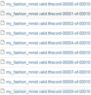
train_filepaths 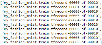
Then use tf.data to create an efficient dataset for each set.
def preprocess(tfrecord):

    feature_descriptions = {
        "image": tf.io.FixedLenFeature([], tf.string, default_value=""), #OR tf.io.VarLenFeature(tf.string)
        "label": tf.io.FixedLenFeature([], tf.int64, default_value=-1)
    }
    example = tf.io.parse_single_example(tfrecord, feature_descriptions)

    #out_type=tf.uint8 since RGB(0~255,0~255,0~255) and 2^8=256 is enough
    image = tf.io.parse_tensor(example["image"], out_type=tf.uint8) # since image_data = tf.io.serialize_tensor(image)
    # image = tf.io.decode_jpeg(example["image"]) # since image_data = tf.io.encode_jpeg( image[..., np.newaxis] )

    image = tf.reshape(image, shape=[28,28]) # <== image[:,:, np.newaxis].shape ==> (28, 28, 1)
    return image, example["label"]

#read data from tfrecords files
def mnist_dataset(filepaths,
                  n_read_threads=5, # num_parallel_reads
                  shuffle_buffer_size=None,
                  n_parse_threads=5,
                  batch_size=5,
                  cache=True):

    dataset = tf.data.TFRecordDataset(filepaths, num_parallel_reads=n_read_threads)

    if cache:
        dataset = dataset.cache()

    if shuffle_buffer_size:
        dataset = dataset.shuffle(shuffle_buffer_size)

    dataset = dataset.map(preprocess, num_parallel_calls=n_parse_threads) #for each record
    dataset = dataset.batch(batch_size)
    return dataset.prefetch(1)

train_set = mnist_dataset(train_filepaths, shuffle_buffer_size=60000)
valid_set = mnist_dataset(valid_filepaths)
test_set = mnist_dataset(test_filepaths)train_set.take(1)image = tf.io.parse_tensor(example["image"], out_type=tf.uint8) # since image_data = tf.io.serialize_tensor(image)
![]()
################################################################ VS tensorflow_datasets
import tensorflow_datasets as tfds

fashion_mnist_bldr=tfds.builder('fashion_mnist')

# Download the data, prepare it, and write it to disk
fashion_mnist_bldr.download_and_prepare()

# Load data from disk as tf.data.Datasets
fashion_mnist_datasets = fashion_mnist_bldr.as_dataset(shuffle_files=False)

fashion_mnist_datasets.keys()![]()
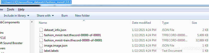
C:\Users\LlQ\tensorflow_datasets\fashion_mnist\3.0.1\dataset_info.json
{
  "citation": "@article{DBLP:journals/corr/abs-1708-07747,\n  author    = {Han Xiao and\n               Kashif Rasul and\n               Roland Vollgraf},\n  title     = {Fashion-MNIST: a Novel Image Dataset for Benchmarking Machine Learning\n               Algorithms},\n  journal   = {CoRR},\n  volume    = {abs/1708.07747},\n  year      = {2017},\n  url       = {http://arxiv.org/abs/1708.07747},\n  archivePrefix = {arXiv},\n  eprint    = {1708.07747},\n  timestamp = {Mon, 13 Aug 2018 16:47:27 +0200},\n  biburl    = {https://dblp.org/rec/bib/journals/corr/abs-1708-07747},\n  bibsource = {dblp computer science bibliography, https://dblp.org}\n}",
  "description": "Fashion-MNIST is a dataset of Zalando's article images consisting of a training set of 60,000 examples and a test set of 10,000 examples. Each example is a 28x28 grayscale image, associated with a label from 10 classes.",
  "downloadSize": "30878645",
  "location": {
    "urls": [
      "https://github.com/zalandoresearch/fashion-mnist"
    ]
  },
  "name": "fashion_mnist",
  "splits": [
    {
      "name": "test",
      "numBytes": "5470824",
      "shardLengths": [
        "10000"
      ]
    },
    {
      "name": "train",
      "numBytes": "32717636",
      "shardLengths": [
        "60000"
      ]
    }
  ],
  "supervisedKeys": {
    "input": "image",
    "output": "label"
  },
  "version": "3.0.1"
}C:\Users\LlQ\tensorflow_datasets\fashion_mnist\3.0.1\image.image.json
{"encoding_format": "png", "shape": [28, 28, 1]}import tensorflow as tf
fashion_mnist__train = fashion_mnist_datasets['train']
assert isinstance(fashion_mnist__train, tf.data.Dataset)
fashion_mnist__train.take(1)![]()
fashion_mnist__train_set = mnist_dataset(r'C:\Users\LlQ\tensorflow_datasets\fashion_mnist\3.0.1\fashion_mnist-train.tfrecord-00000-of-00001')
fashion_mnist__train_set.take(1)![]()
################################################################
import matplotlib.pyplot as plt

for X,y in train_set.take(1):
    for i in range(5):
        plt.subplot(1,5, i+1)
        plt.imshow(X[i].numpy(), cmap="binary")
        plt.axis("off")
        plt.title(str(y[i].numpy()))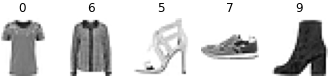
Finally, use a Keras model to train these datasets, including a preprocessing layer to standardize each input feature. Try to make the input pipeline as efficient as possible, using TensorBoard to visualize profiling data.
keras.backend.clear_session()
tf.random.set_seed(42)
np.random.seed(42)

class Standardization(keras.layers.Layer):
    def adapt(self, data_sample):
        self.means_ = np.mean(data_sample, axis=0, keepdims=True)
        self.stds_ = np.std(data_sample, axis=0, keepdims=True)

    def call(self, inputs):
        return (inputs-self.means_) / (self.stds_ + keras.backend.epsilon())

standardization = Standardization(input_shape=[28,28])
sample_image_batches = train_set.map(lambda image, label: image)
sample_images = np.concatenate(list(sample_image_batches.as_numpy_iterator()),
                               axis=0).astype(np.float32)
#len(sample_images) == 5 * 100 batches
standardization.adapt(sample_images)

model = keras.models.Sequential([
    standardization,
    keras.layers.Flatten(), #1D
    keras.layers.Dense(100, activation="relu"),
    keras.layers.Dense(10, activation="softmax")
])
model.compile(loss="sparse_categorical_crossentropy", optimizer='nadam',
              metrics=["accuracy"])
from datetime import datetime
import os
import math
logs = os.path.join(os.curdir, "my_logs", "run_"+datetime.now().strftime("%Y%m%d_%H%M%S"))
tensorboard_cb = tf.keras.callbacks.TensorBoard(log_dir=logs,
histogram_freq=1,
profile_batch=10)
batch_size=32 #default
model.fit(train_set, steps_per_epoch=np.ceil(len(X_train)/batch_size),
epochs=5,
validation_data=valid_set, callbacks=[tensorboard_cb])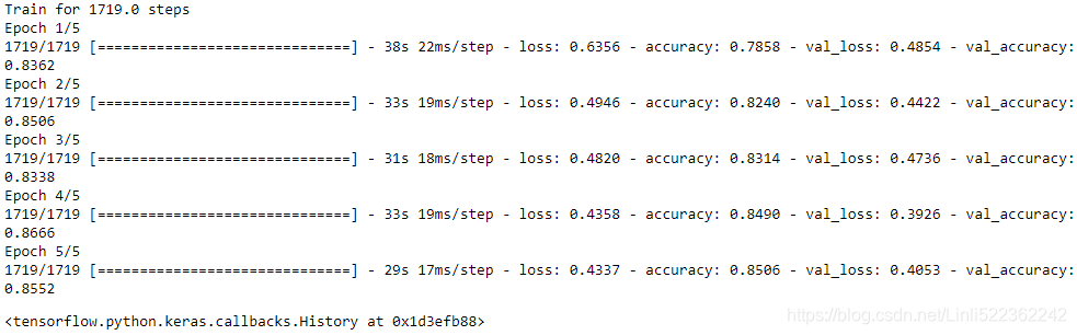
Warning: The profiling tab in TensorBoard works if you use TensorFlow 2.2+. You also need to make sure tensorboard_plugin_profile is installed (and restart Jupyter if necessary).![]()
%load_ext tensorboard
%tensorboard --logdir=./my_logs --port=6006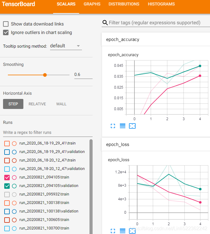
Reason: No GPU
device_name = tf.test.gpu_device_name()
if not device_name:
  raise SystemError('GPU device not found')
print('Found GPU at: {}'.format(device_name))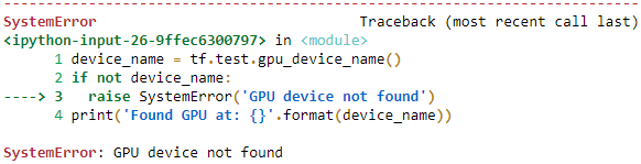
################################################################################
################################################################################
10. In this exercise you will download a dataset, split it, create a tf.data.Dataset to load it and preprocess it efficiently, then build and train a binary classification model containing an Embedding layer:
- a. Download the Large Movie Review Dataset http://ai.stanford.edu/~amaas/data/sentiment/, which contains 50,000 movies reviews from the Internet Movie Database. The data is organized in two directories, train and test, each containing a pos subdirectory with 12,500 positive reviews and a neg subdirectory with 12,500 negative reviews. Each review is stored in a separate text file. There are other files and folders (including preprocessed bag-of-words), but we will ignore them in this exercise.
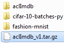
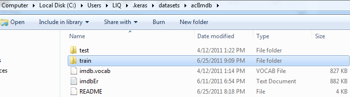
from pathlib import Path from tensorflow import keras DOWNLOAD_ROOT = "http://ai.stanford.edu/~amaas/data/sentiment/" FILENAME = "aclImdb_v1.tar.gz" filepath = keras.utils.get_file(FILENAME, DOWNLOAD_ROOT + FILENAME, extract=True) path = Path(filepath).parent / "aclImdb" path -
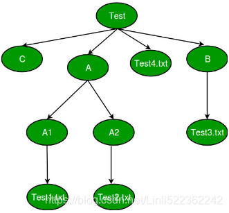
Unzipped file directory tree
OS.walk() generate the file names in a directory tree by walking the tree either top-down or bottom-up. For each directory in the tree rooted at directory top (including top itself), it yields a 3-tuple (dirpath, dirnames, filenames).
root : Prints out directories only from what you specified.
dirs : Prints out sub-directories from root.
files : Prints out all files from root and directories.# Driver function import os if __name__ == "__main__": for (root,dirs,files) in os.walk('Test', topdown=true): print root print dirs print files print '--------------------------------'
path.parts
import os

#name: current directory OR folder
for name, subdirs, files in os.walk(path):
    indent = len(Path(name).parts) - len(path.parts)
    print("    " *indent + Path(name).parts[-1] + os.sep)
    for index, filename in enumerate( sorted(files) ):
        if index == 3:
            print("    " *(indent+1) + "...")
            break; #exist for loop
        print("    " *(indent+1) + filename)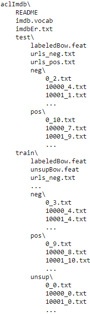
-
Files Access path
def review_paths(dirpath):
    return [str(path) for path in dirpath.glob("*.txt")]

train_pos = review_paths(path / "train" / "pos") # WindowsPath('C:/Users/LlQ/.keras/datasets/aclImdb/train/pos')
train_neg = review_paths(path / "train" / "neg")

test_valid_pos = review_paths(path / "test" / "pos")
test_valid_neg = review_paths(path / "test" / "neg")

len(train_pos), len(train_neg), len(test_valid_pos), len(test_valid_neg)
 ==>
==>
- b. Split the test set into a validation set (15,000) and a test set (10,000).
import numpy as np np.random.shuffle(test_valid_pos) test_pos = test_valid_pos[:5000] test_neg = test_valid_neg[:5000] valid_pos = test_valid_pos[5000:] valid_neg = test_valid_neg[5000:] - c. Use tf.data to create an efficient dataset for each set.
Since the dataset fits in memory, we can just load all the data using pure Python code and usetf.data.Dataset.from_tensor_slices(): # reading all filesimport tensorflow as tf def imdb_dataset(filepaths_positive, filepaths_negative): reviews = [] labels = [] for filepaths, label in ( (filepaths_negative, 0), (filepaths_positive, 1) ): for filepath in filepaths: with open(filepath, encoding="utf8") as review_file: reviews.append( review_file.read() ) labels.append(label) return tf.data.Dataset.from_tensor_slices( ( tf.constant(reviews), tf.constant(labels) ) ) for X,y in imdb_dataset(train_pos, train_neg).take(1): print(X) print(y) print()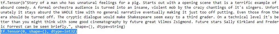

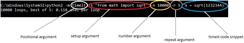
%timeit -r1 for X, y in imdb_dataset(train_pos, train_neg).repeat(10): pass
It takes about 1 minute 26 seconds to load the dataset and go through it 10 times.
-
TFRecords
But let's pretend the dataset does not fit in memory, just to make things more interesting. Luckily, each review fits on just one line (they use<br />to indicate line breaks), so we can read the reviews using aTextLineDataset. If they didn't we would have to preprocess the input files (e.g., converting them to TFRecords). For very large datasets, it would make sense a tool like Apache Beam for that. # reading data batch by batch and multiple parallelsdef imdb_dataset(filepaths_positive, filepaths_negative, n_read_threads=5): dataset_neg = tf.data.TextLineDataset( filepaths_negative, num_parallel_reads=n_read_threads ) dataset_neg = dataset_neg.map( lambda review: (review, 0) ) dataset_pos = tf.data.TextLineDataset( filepaths_positive, num_parallel_reads=n_read_threads ) dataset_pos = dataset_pos.map( lambda review: (review, 1) ) return tf.data.Dataset.concatenate( dataset_pos, dataset_neg ) %timeit -r1 for X,y in imdb_dataset(train_pos, train_neg).repeat(10): pass
Now it takes about 2 minutes 54 seconds to go through the dataset 10 times. That's much slower, essentially because the dataset is not cached in RAM, so it must be reloaded at each epoch. If you add
.cache()just before.repeat(10), you will see that this implementation will be about as fast as the previous one.%timeit -r1 for X,y in imdb_dataset(train_pos, train_neg).cache().repeat(10): pass
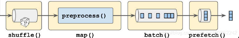
batch_size = 32 train_set = imdb_dataset(train_pos, train_neg).shuffle(25000).batch(batch_size).prefetch(1) valid_set = imdb_dataset(valid_pos, valid_neg).batch(batch_size).prefetch(1) test_set = imdb_dataset(test_pos, test_neg).batch(batch_size).prefetch(1) for X,y in train_set.take(1): print(X)# print(len(X)) # 32 print(y)# print(len(y)) # 32 print() 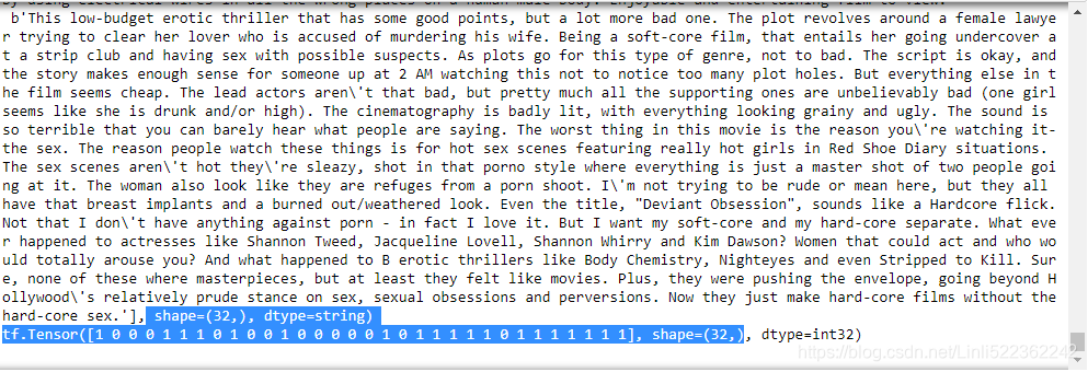
- d. Create a binary classification model, using a TextVectorization layer to preprocess each review. If the TextVectorization layer is not yet available (or if you like a challenge), try to create your own custom preprocessing layer: you can use the functions in the tf.strings package, for example lower() to make everything lowercase, regex_replace() to replace punctuation with spaces, and split() to split words on spaces. You should use a lookup table to output word indices, which must be prepared in the adapt() method.
Let's first write a function to preprocess the reviews, cropping them to 300 characters, converting them to lower case, then replacing<br />and all non-letter characters to spaces, splitting the reviews into words, and finally padding or cropping each review so it ends up with exactlyn_wordstokens:
#################################################
https://blog.csdn.net/Linli522362242/article/details/87780336
https://blog.csdn.net/Linli522362242/article/details/90139705
https://blog.csdn.net/Linli522362242/article/details/103866244<br /> ==> "<br\\s*/?>"
all non-letter characters ==> b"[^a-z]"X_example = tf.constant(["It's a great, great movie! I loved it.", "It was terrible, run away!!!"]) tf.shape(X_example)
tf.shape(X_example)*tf.constant([1,0])
tf.shape(X_example)*tf.constant([1,0])+ tf.constant([0, 50])
################################################# -
tokenizer
-
def preprocess(X_batch, n_words=50):
    shape = tf.shape(X_batch) * tf.constant([1,0]) + tf.constant([0, n_words])# ==> shape(batches, n_words)
    Z = tf.strings.substr(X_batch, 0, 300) # cropping them to 300 characters

    # <head.*?>   matches only one “<head>”
    Z = tf.strings.lower(Z)                              # "\" : An escape character
    Z = tf.strings.regex_replace(Z, b"<br\\s*/?>", b" ") # "\s": white space, "\S": non-white space OR ([^\s])
    Z = tf.strings.regex_replace(Z, b"[^a-z]", b" ") # replace all non-letter characters to spaces
    Z = tf.strings.split(Z) #splitting the reviews into words

    return Z.to_tensor(shape=shape, default_value=b"<pad>")

X_example = tf.constant(["It's a great, great movie! I loved it.", "It was terrible, run away!!!"])
preprocess(X_example)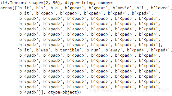
Now let's write a second utility function that will take a data sample with the same format as the output of thepreprocess()function, and will output the list of the topmax_sizemost frequent words, ensuring that the padding token is first:
-
get_vocabulary
from collections import Counter

def get_vocabulary( data_sample, max_size=1000):
    preprocess_reviews = preprocess(data_sample).numpy()
    counter = Counter()

    for words in preprocess_reviews:
        for word in words:
            if word != b"<pad>" :
                counter[word] += 1
    return [b"<pad>"] + [word for word, count in counter.most_common(max_size)]

get_vocabulary(X_example)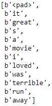
Now we are ready to create theTextVectorizationlayer. Its constructor just saves the hyperparameters (max_vocabulary_sizeandn_oov_buckets). Theadapt()method computes the vocabulary using theget_vocabulary()function, then it builds aStaticVocabularyTable(see Chapter 16 for more details). Thecall()method preprocesses the reviews to get a padded list of words for each review, then it uses theStaticVocabularyTableto lookup the index of each word in the vocabulary:
self.n_oov_buckets: specify the number of out-of-vocabulary (oov) buckets. If we look up a category that does not exist in the vocabulary, the lookup table will compute a hash of this category and use it to assign the unknown category to one of the oov buckets. -
TextVectorization
class TextVectorization(keras.layers.Layer):
    def __init__(self, max_vocabulary_size=1000, n_oov_buckets=100, dtype=tf.string, **kwargs):
        super().__init__(dtype=dtype, **kwargs)
        self.max_vocabulary_size = max_vocabulary_size
        self.n_oov_buckets = n_oov_buckets

    def adapt(self, data_sample):
        self.vocab = get_vocabulary(data_sample, self.max_vocabulary_size)
        words = tf.constant(self.vocab)
        word_ids = tf.range( len(self.vocab), dtype=tf.int64 )

        # https://blog.csdn.net/Linli522362242/article/details/107933572
        vocab_init = tf.lookup.KeyValueTensorInitializer(words, word_ids)
        self.table = tf.lookup.StaticVocabularyTable(vocab_init, self.n_oov_buckets) # builds a StaticVocabularyTable

    def call(self, inputs):
        preprocessed_inputs = preprocess(inputs) #reviews ==> words array
        return self.table.lookup(preprocessed_inputs)
Let's try it on our small
X_examplewe defined earlier:text_vectorization = TextVectorization() text_vectorization.adapt(X_example) text_vectorization(X_example)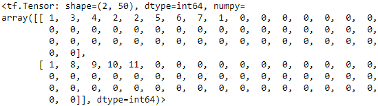
Looks good! As you can see, each review was cleaned up and tokenized, then each word was encoded as its index in the vocabulary (all the 0s correspond to the<pad>tokens)
Now let's create anotherTextVectorizationlayer and let's adapt it to the full IMDB training set (if the training set did not fit in RAM, we could just use a smaller sample of the training set by callingtrain_set.take(500)):max_vocabulary_size = 1000 n_oov_buckets = 100 sample_review_batches = train_set.map(lambda review, label: review) #tensor: [batch, batch, ...] sample_reviews = np.concatenate( list( sample_review_batches.as_numpy_iterator() ), axis=0) # to one list text_vectorization = TextVectorization(max_vocabulary_size, n_oov_buckets, input_shape=[]) text_vectorization.adapt(sample_reviews) text_vectorization(X_example)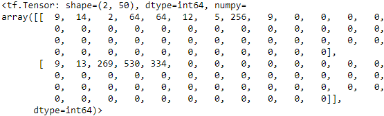
Good! Now let's take a look at the first 10 words in the vocabulary:text_vectorization.vocab[:10]
These are the most common words in the reviews.
-
bags of words
Now to build our model we will need to encode all these word IDs somehow. One approach is to create bags of words: for each review, and for each word in the vocabulary, we count the number of occurences of that word in the review. For example:simple_example = tf.constant([ [1,3,1,0,0], [2,2,0,0,0] ]) tf.one_hot(simple_example, 4)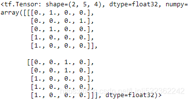
simple_example = tf.constant([ [1,3,1,0,0],
                               [2,2,0,0,0] ])
tf.reduce_sum( tf.one_hot(simple_example, 4), axis=1)
<tf.Tensor: shape=(2, 4), dtype=float32, numpy=
array([[2., 2., 0., 1.], # since two-0s, two-1s, no 2, one-3s
[3., 0., 2., 0.]], dtype=float32)> # since three-0s, no 1, two-2s, no 3
The first review has 2 times the word 0, 2 times the word 1, 0 times the word 2, and 1 time the word 3, so its bag-of-words representation is [2, 2, 0, 1]. Similarly, the second review has 3 times the word 0, 0 times the word 1, and so on.
Let's wrap this logic in a small custom layer, and let's test it. We'll drop the counts for the word 0, since this corresponds to the <pad> token, which we don't care about.class BagOfWords(keras.layers.Layer): def __init__(self, n_tokens, dtype=tf.int32, **kwargs): super().__init__(dtype=tf.int32, **kwargs) self.n_tokens = n_tokens def call(self, inputs): one_hot = tf.one_hot(inputs, self.n_tokens) return tf.reduce_sum(one_hot, axis=1) [:,1:] # Let's test it: bag_of_words = BagOfWords(n_tokens=4) bag_of_words( simple_example ) 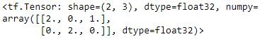
It works fine! Now let's create anotherBagOfWordwith the right vocabulary size for our training set:
We're ready to train the model!n_tokens = max_vocabulary_size + n_oov_buckets + 1 # add 1 for <pad> bag_of_words = BagOfWords(n_tokens)
keras.backend.clear_session()
tf.random.set_seed(42)
np.random.seed(42)

model = keras.models.Sequential([
    text_vectorization,
    bag_of_words,
    keras.layers.Dense(100, activation="relu"),
    keras.layers.Dense(1, activation="sigmoid"),
])

model.compile(loss="binary_crossentropy", optimizer="nadam", metrics=["accuracy"])
model.fit(train_set, epochs=5, validation_data=valid_set)
We get about 73.5% accuracy on the validation set after just the first epoch, but after that the model makes no progress. We will do better in Chapter 16. For now the point is just to perform efficient preprocessing usingtf.dataand Keras preprocessing layers.-
Embedding
-
e. Add an Embedding layer and compute the mean embedding for each review, multiplied by the square root of the number of words (see Chapter 16). This rescaled mean embedding can then be passed to the rest of your model.
-
To be precise, the sentence(here, one sentence per review) embedding is equal to the mean word embedding multiplied by the square root of the number of words in the sentence. This compensates for the fact that the mean of n vectors gets shorter as
n grows.
To compute the mean embedding for each review, and multiply it by the square root of the number of words in that review, we will need a little function:# another_example[review1[ 1_word_dimesions[], 1_word_dimesions[], 1_word_dimensions[] ], # review2[ 1_word_dimesions[], 1_word_dimesions[], 1_word_dimensions[] ] # ] #d1 d2 d3 # another_example = tf.constant([ [ [1., 2., 3.], # word # [4., 5., 0.], # word # [0., 0., 0.] # word # ],# one sentence(1 line) represents one review # [ [6., 0., 0.], # [0., 0., 0.], # [0., 0., 0.] # ] # ]) # # not_pad = tf.math.count_nonzero(inputs, axis=-1)######################## # tf.math.count_nonzero(another_example, axis=-1) # <tf.Tensor: shape=(2, 3), dtype=int64, numpy= # array([[3, 2, 0], # [1, 0, 0]], dtype=int64)> # # n_words = tf.math.count_nonzero(not_pad, axis=-1, keepdims=True)######## # tf.math.count_nonzero(tf.math.count_nonzero(another_example, axis=-1), # axis=-1, # keepdims=True) # <tf.Tensor: shape=(2, 1), dtype=int64, numpy= # array([[2], # [1]], dtype=int64)> #The first review contains 2 words (the last token is a zero vector, #which represents the <pad> token). The second review contains 1 word. # # sqrt_n_words = tf.math.sqrt( tf.cast(n_words, tf.float32) )############## # tf.math.sqrt( tf.cast(tf.math.count_nonzero(tf.math.count_nonzero(another_example, axis=-1), # axis=-1, # keepdims=True), tf.float32) ) # <tf.Tensor: shape=(2, 1), dtype=float32, numpy= # array([[1.4142135], # [1. ]], dtype=float32)> # # return tf.reduce_mean(inputs, axis=1) * sqrt_n_words #################### # tf.reduce_mean(another_example, axis=1) # <tf.Tensor: shape=(2, 3), dtype=float32, numpy= # mean word embedding , mean word embedding , mean word embedding # array([[ 1.6666666==(1+4+0)/3, 2.3333333==(2+5+0)/3, 1.==(3+0+0)/3 words ], # [ 2. ==(6+0+0)/3, 0. ==(0+0+0)/3, 0.==(0+0+0)/3 ] # ], dtype=float32)> # 1.4142135*1.6666666 = 2.3570224 # 1.4142135*2.3333333 = 3.2998314 # tf.reduce_mean(another_example, axis=1) * tf.math.sqrt( tf.cast(tf.math.count_nonzero(tf.math.count_nonzero(another_example, axis=-1), # axis=-1, # keepdims=True), # tf.float32) # ) # <tf.Tensor: shape=(2, 3), dtype=float32, numpy= # array([[2.3570225, 3.2998314, 1.4142135], # [2. , 0. , 0. ]], dtype=float32)> def compute_mean_embedding(inputs): not_pad = tf.math.count_nonzero(inputs, axis=-1) n_words = tf.math.count_nonzero(not_pad, axis=-1, keepdims=True) sqrt_n_words = tf.math.sqrt( tf.cast(n_words, tf.float32) ) return tf.reduce_mean(inputs, axis=1) * sqrt_n_words another_example = tf.constant([ [ [1., 2., 3.], [4., 5., 0.], [0., 0., 0.] ], [ [6., 0., 0.], [0., 0., 0.], [0., 0., 0.] ] ]) compute_mean_embedding(another_example)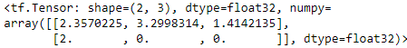
Let's check that this is correct. The first review contains 2 words (the last token is a zero vector, which represents the<pad>token). The second review contains 1 word. So we need to compute the mean embedding for each review, and multiply the first one by the square root of 2, and the second one by the square root of 1:tf.reduce_mean( another_example, axis=1) * tf.sqrt([[2.], [1.] ]) -
Perfect. Now we're ready to train our final model. It's the same as before, except we replaced the
BagOfWordslayer with anEmbeddinglayer followed by aLambdalayer that calls thecompute_mean_embeddinglayer:embedding_size=20 model = keras.models.Sequential([ text_vectorization, keras.layers.Embedding(input_dim=n_tokens, #n_tokens = max_vocabulary_size + n_oov_buckets + 1 # add 1 for <pad> output_dim=embedding_size, mask_zero=True), # <pad> tokens => zero vectors keras.layers.Lambda(compute_mean_embedding), keras.layers.Dense(100, activation="relu"), keras.layers.Dense(1, activation="sigmoid") ]) - f. Train the model and see what accuracy you get. Try to optimize your pipelines to make training as fast as possible.
model.compile(loss="binary_crossentropy", optimizer="nadam", metrics=["accuracy"])
model.fit(train_set, epochs=5, validation_data= valid_set)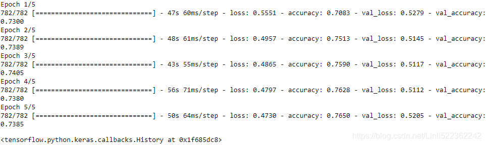
The model is not better using embeddings (but we will do better in Chapter 16). The pipeline looks fast enough (we optimized it earlier). - g. Use TFDS to load the same dataset more easily: tfds.load("imdb_reviews").
import tensorflow_datasets as tfds

datasets = tfds.load(name="imdb_reviews")
train_set, test_set = datasets["train"], datasets["test"]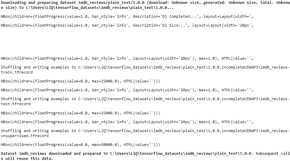
for example in train_set.take(1):
    print(example["text"])
    print(example["label"])


 264
264


 被折叠的 条评论
为什么被折叠?
被折叠的 条评论
为什么被折叠?
 到【灌水乐园】发言


