14_4计算机视觉 Fully Conv dense_mnist_compute parameters_run out of RAMemo_local response normal_Semantic

14_Deep Computer Vision Using Convolutional Neural Networks_max pool_GridSpec_tf.nn, layers, contrib:
https://blog.csdn.net/Linli522362242/article/details/108302266

14_Deep Computer Vision Using Convolutional Neural Networks_2_LeNet-5_ResNet-50_ran out of data_Augmentation_skip_countplot_shape_crop_and_resize
https://blog.csdn.net/Linli522362242/article/details/108396485

14_Deep Computer Vision Using Convolutional Neural Networks_3_CNN_dense_v1_v2_YOLO_meanAveragePrecision_mAP_bilinear_resize image_tf.nn.Conv2DTranspose_dilation_flip
https://blog.csdn.net/Linli522362242/article/details/108669444

1. What are the advantages of a CNN over a fully connected DNN for image classification?

################################################### https://blog.csdn.net/Linli522362242/article/details/111940633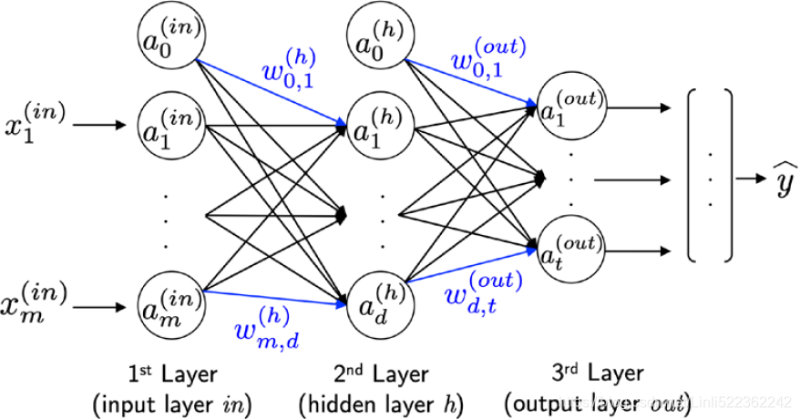
 The MLP(Multilayer Perceptron) depicted in the preceding figure has one input layer, one hidden layer, and one output layer. The units in the hidden layer are fully connected to the input layer, and the output layer is fully connected to the hidden layer. If such a network has more than one hidden layer, we also call it a deep artificial NN.
########### https://blog.csdn.net/Linli522362242/article/details/108414534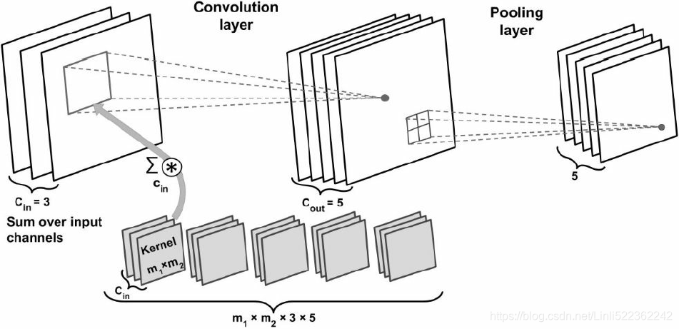
    In this example input tensor is of size , there are three input channels. The kernel tensor is four dimensional . Each kernel matrix is denoted as , and there are three of them, one for each input channel. Furthermore, there are five such kernels, accounting for five output feature maps. Finally, there is a pooling layer for subsampling the feature maps, as shown in the figure.

How many trainable parameters exist in the preceding example?
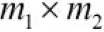
     To illustrate the advantages of convolution, parameter-sharing and sparse connectivity, let's work through an example. The convolutional layer in the network shown in the preceding figure is a four-dimensional tensor. So, there are  parameters associated with the kernel. Furthermore, there is a bias vector for each output feature map of the convolutional layer. Thus, the size of the bias vector is 5 . Pooling layers do not have any (trainable) parameters; therefore, we can write the following:
 (+5 since the bias vector)

     If input tensor is of size , assuming that the convolution is performed with mode='same', then the output feature maps would be of size .
     Note that this number is much smaller than the case if we wanted to have a fully connected layer instead of the convolution layer. In the case of a fully connected layer, the number of parameters for the weight matrix to reach the same number of output units would have been as follows:

     In addition, the size of the bias vector is  (one bias element for each output unit). Given that  and , we can see that the difference in the number of trainable parameters is huge.

##########Memory Requirementshttps://blog.csdn.net/Linli522362242/article/details/108302266
     For example, consider a convolutional layer with 5 × 5 ( == x  ) filters, outputting 200 feature maps of size 150 × 100, with stride 1 and "same" padding. If the input is a 150 × 100 RGB image (three channels), then the number of parameters is (5 × 5 × 3 + 1) × 200 = 15,200 (the + 1 corresponds to the bias terms, and 3 possible sets of weights OR (5 × 5 × 3 × 200 + 200), which is fairly small compared to a fully connected layer
(###A fully connected layer with 150 × 100 neurons(the size of each output feature map: 150 × 100), each connected to all 150 × 100 × 3 inputs, would have 150^2× 100^2 × 3 = 675 million(OR 675,000,000) parameters! x200 since the output contains 200 feature maps;
Thus, (50 × 100)^2 × 3 x 200
###).
However, each of the 200 feature maps(output) contains 150 × 100 neurons, and each of these neurons needs to compute a weighted sum of its 5 × 5 × 3 = 75 inputs: that’s a total of 225 million float multiplications(225, 000, 000=75 inputs * 150*100 neurons*200 feature maps). Not as bad as a fully connected layer, but still quite computationally intensive(for convolutional layer). Moreover, if the feature maps are represented using 32-bit floats, then the convolutional layer’s output will occupy 200 × 150 × 100 × 32 = 96 million bits (12 MB) of RAM(In the international system of units (SI), 1 MB = 1,000 KB = 1,000 × 1,000 bytes = 1,000 × 1,000 × 8 bits.). And that’s just for one instance—if a training batch contains 100 instances, then this layer will use up 1.2 GB of RAM!

#########################partially connected

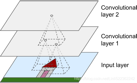Figure 14-2. CNN layers with rectangular local receptive fields

     The most important building block of a CNN is the convolutional layer: neurons in the first convolutional layer (Convolutional layer 1) are not connected to every single pixel in the input image(Input layer) (like they were in the layers discussed in previous chapters), but only to pixels in their receptive fields ( in Input layer)(see Figure 14-2). In turn, each neuron in the second convolutional layer is connected only to neurons located within a small rectangle in the first layer. This architecture allows the network to concentrate on small low-level features in the first hidden layer, then assemble them into larger higher-level features in the next hidden layer, and so on. This hierarchical structure is common in real-world images, which is one of the reasons why CNNs work so well for image recognition.
###################################################

     These are the main advantages of a CNN(Convolutional Neural Network) over a fully connected DNN(A fully connected neural network) for image classification:

• • Because consecutive layers are only partially connected and because it heavily reuses its weights(use same kernel matrix  on each input feature map), a CNN has many fewer parameters than a fully connected DNN, which makes it much faster to train, reduces the risk of overfitting, and requires much less training data.
• • When a CNN has learned a kernel that can detect a particular feature, it can detect that feature anywhere in the image. In contrast, when a DNN learns a feature in one location, it can detect it only in that particular location. Since images typically have very repetitive features, CNNs are able to generalize much better than DNNs for image processing tasks such as classification, using fewer training examples.
   
• • Finally, a DNN has no prior knowledge of how pixels are organized; it does not know that nearby pixels are close. A CNN’s architecture embeds this prior knowledge. Lower layers typically identify features in small areas of the images, while higher layers combine the lower-level features into larger features. This works well with most natural images, giving CNNs a decisive head start compared to DNNs.

2. Consider a CNN composed of three convolutional layers, each with 3 × 3 kernels, a stride of 2, and "same" padding. The lowest layer outputs 100 feature maps, the middle one outputs 200, and the top one outputs 400. The input images are RGB images of 200 × 300 pixels. What is the total number of parameters in the CNN? If we are using 32-bit floats, at least how much RAM will this network require when making a prediction for a single instance? What about when training on a mini-batch of 50 images?

     ############### Let’s compute how many parameters the CNN has. Since its

1. first convolutional layer has 3 × 3 kernels, and the input has three channels (red, green, and blue), each feature map has 3 × 3 × 3 weights, plus a bias term. That’s 28 parameters per feature map. Since this first convolutional layer outputs 100 feature maps, it has a total of 2,800 parameters( (3x3x3+1)x100).
    
2. The second convolutional layer has 3 × 3 kernels and its input is the set of 100 feature maps of the previous layer, so each feature map has 3 × 3 × 100 = 900 weights, plus a bias term. Since it outputs 200 feature maps, this layer has 901 × 200 = 180,200 parameters( (3x3x100+1)x200).
    
3. Finally, the third and last convolutional layer also has 3 × 3 kernels, and its input is the set of 200 feature maps of the previous layers, so each feature map has 3 × 3 × 200 = 1,800 weights, plus a bias term. Since it has 400 feature maps, this layer has a total of 1,801 × 400 =720,400 parameters( (3 × 3 x 200 + 1) × 400).
    
4. All in all, the CNN has 2,800 + 180,200 + 720,400 = 903,400 parameters(!hold).

     ############### Now let’s compute how much RAM this neural network will require (at least) when making a prediction for a single instance.

1. First let’s compute the feature map size for each layer. Since we are using a stride of 2 and "same" padding(==>input dimension ==output dimension if stride=1), the horizontal and vertical dimensions of the feature maps are divided by 2 at each layer (rounding up if necessary).
   1. So, as the input channels are 200 × 300 pixels, the first layer’s feature maps are 100 × 150 (### 100 = 200/2 and 150=300/2 ###),
   2. the second layer’s feature maps are 50 × 75 (### 50 = 100/2 and 75=150/2 ###), and
   3. the third layer’s feature maps are 25 × 38 (### 25 = 50/2 and 38=75/2=37.5 ==>np.ceil==>38 ###).
       
   4. Since 32 bits is 4 bytes (### 4 bytes= 32/8bits per byte ###) and the first convolutional layer outputs 100 feature maps,
      
      this first layer takes up 4 × 100 × 150 × 100 = 6 million bytes (6 MB=6,000 KB x1000 Bytes, outputs 100 feature maps).
      The second layer takes up 4 × 50 × 75 × 200 = 3 million bytes (3 MB=3,000 KB x 1000 Bytes, outputs 200 feature maps).
      Finally, the third layer takes up 4 × 25 × 38 × 400 = 1,520,000 bytes (1.52 MB=1,520 KB x 1000 Bytes, outputs 200 feature maps).
2. However, once a layer has been computed, the memory occupied by the previous layer can be released, so if everything is well optimized, only 6 + 3 = 9 million bytes (9 MB) of RAM will be required (when the second layer has just been computed, but the memory occupied by the first layer has not been released yet).
    
3. But wait, you also need to add the memory occupied by the CNN’s parameters! We computed earlier that it has 903,400 parameters, each using up 4 bytes(since using 32-bit floats), so this adds 3,613,600 bytes (about 3.6 MB, 3,613,600 bytes=903,400 x 4 bytes).
    
4. The total RAM required is therefore (at least) 12,613,600 bytes (about 12.6 MB).

     Lastly, let’s compute the minimum amount of RAM required when training the CNN on a mini-batch of 50 images. During training TensorFlow uses backpropagation, which requires keeping all values computed during the forward pass until the reverse pass begins. So we must compute the total RAM required by all layers for a single instance and multiply that by 50. At this point, let’s start counting in megabytes rather than bytes.

• We computed before that the three layers require respectively 6, 3, and 1.52 MB for each instance. That’s a total of 10.52 MB per instance, so for 50 instances the total RAM required is 526 MB.
• Add to that the RAM required by the input images, which is 50 × 200 × 300 × 3 × 4 = 36 million bytes (36 MB, 50 instances, 200x300 pixels, 3 channels, 4 bytes ),
• plus the RAM required for the model parameters, which is about 3.6 MB (computed earlier),
• plus some RAM for the gradients (we will neglect this since it can be released gradually as backpropagation goes down the layers during the reverse pass).
• We are up to a total of roughly 526 + 36 + 3.6 = 565.6 MB, and that’s really an optimistic bare minimum.

3. If your GPU runs out of memory while training a CNN, what are five things you could try to solve the problem?

     If your GPU runs out of memory while training a CNN, here are five things you could try to solve the problem (other than purchasing a GPU with more RAM):

• • Reduce the mini-batch size.
• • Reduce dimensionality using a larger stride in one or more layers.
• • Remove one or more layers.
• • Use 16-bit floats instead of 32-bit floats.
• • Distribute the CNN across multiple devices.

4. Why would you want to add a max pooling layer rather than a convolutional layer with the same stride?

     A max pooling layer has no parameters at all, whereas a convolutional layer has quite a few (see the previous questions).

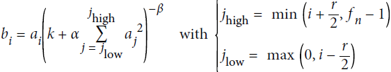
5. When would you want to add a local response normalization layer?

     A local response normalization layer makes the neurons that most strongly activate inhibit抑制 neurons at the same location but in neighboring feature maps, which encourages different feature maps to specialize and pushes them apart, forcing them to explore a wider range of features. It is typically used in the lower layers to have a larger pool of low-level features that the upper layers can build upon.
################# https://blog.csdn.net/Linli522362242/article/details/108396485

and
 

In this equation:

•  is the normalized output of the neuron located in feature map i, at some row u and column v (note that in this equation we consider only neurons located at this row and column, so u and v are not shown).
• is the activation of that neuron after the ReLU step, but before normalization.
• k, α, β, and r are hyperparameters. k is called the bias, and r is called the depth radius(OR r “adjacent” kernel maps at the same spatial position).
• is the number of feature maps.

     For example, if r = 2 and a neuron has a strong activation, it will inhibit the activation of the neurons located in the feature maps immediately above( i+2/2=i+1) and below( i-2/2=i-1 ) its own.
################# https://blog.csdn.net/Linli522362242/article/details/108396485

6. Can you name the main innovations in AlexNet, compared to LeNet-5? What about the main innovations in GoogLeNet, ResNet, SENet, and Xception?
 
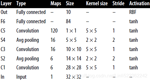
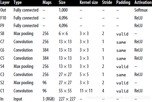
Table 14-1. LeNet-5 architecture                        Table 14-2. AlexNet architecture

     The main innovations in AlexNet compared to LeNet-5 are that it is much larger and deeper, and it stacks convolutional layers(C5, C6, C7) directly on top of each other, instead of stacking a pooling layer on top of each convolutional layer.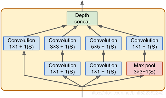
Figure 14-13. Inception
     The main innovation in GoogLeNet is the introduction of inception modules, which make it possible to have a much deeper net than previous CNN architectures, with fewer parameters.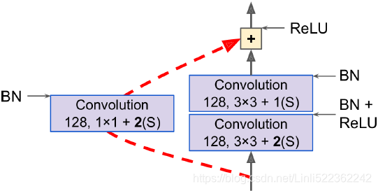
Figure 14-18. Skip connection when changing feature map size(stride 2) and depth (e.g. from 64 to 128)
     ResNet’s main innovation is the introduction of skip connections, which make it possible to go well beyond 100 layers. Arguably, its simplicity and consistency are also rather innovative.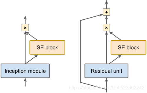
Figure 14-20. SE-Inception module (left) and SE-ResNet unit (right)
     SENet’s main innovation was the idea of using an SE block (a two-layer dense network) after every inception module in an inception network or every residual unit in a ResNet to recalibrate the relative importance of feature maps (###An SE block analyzes the output of the unit it is attached to, focusing exclusively on the depth dimension (it does not look for any spatial pattern), and it learns which features are usually most active together. It then uses this information to recalibrate再校准 the feature maps ###)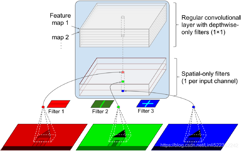
Figure 14-19. Depthwise separable convolutional layer ( too few channels, just for illustration purposes) from bottom to up
Finally, Xception’s main innovation was the use of depthwise separable convolutional layers, which look at spatial patterns and depthwise patterns separately.

7. What is a fully convolutional network? How can you convert a dense layer into a convolutional layer?

     Fully convolutional networks are neural networks composed exclusively of convolutional and pooling layers. FCNs can efficiently process images of any width and height (at least above the minimum size). They are most useful for object detection and semantic segmentation because they only need to look at the image once (instead of having to run a CNN multiple times on different parts of the image). If you have a CNN with some dense layers on top, you can convert these dense layers to convolutional layers to create an FCN:

• just replace the lowest dense layer with a convolutional layer with a kernel size(the filter size) equal to the layer’s input size,
• with one filter per neuron in the dense layer(the number of filters in the convolutional layer must be equal to the number of units in the dense layer), and ==
• using "valid" padding. Generally the stride should be 1, but you can set it to a higher value if you want.
• The activation function should be the same as the dense layer’s. The other dense layers should be converted the same way, but using 1 × 1 filters. It is actually possible to convert a trained CNN this way by appropriately reshaping the dense layers’ weight matrices.

8. What is the main technical difficulty of semantic segmentation?

     The main technical difficulty of semantic segmentation is the fact that a lot of the spatial information gets lost in a CNN as the signal flows through each layer, especially in pooling layers and layers with a stride greater than 1. This spatial information needs to be restored somehow to accurately predict the class of each pixel. https://blog.csdn.net/Linli522362242/article/details/108669444

9. Build your own CNN from scratch and try to achieve the highest possible accuracy on MNIST.

from tensorflow import keras

# https://www.tensorflow.org/api_docs/python/tf/keras/datasets/mnist/load_data
# mnist: This is a dataset of 60,000 28x28 grayscale images of the 10 digits, 
#        along with a test set of 10,000 images.
# X_train_full, X_test: uint8 arrays of grayscale image data with shapes 
# (num_samples, 28, 28).
# y_train_full, y_test: uint8 arrays of digit labels (integers in range 0-9) 
# with shapes (num_samples,).
# unit8 ==> 2^8 = 256 ==> 0.~255.
(X_train_full, y_train_full), (X_test, y_test) = keras.datasets.mnist.load_data()
# Normalization
X_train_full = X_train_full / 255.
X_test = X_test / 255.

X_train, X_valid = X_train_full[:-5000], X_train_full[-5000:]
y_train, y_valid = y_train_full[:-5000], y_train_full[-5000:]
X_train.shape

import numpy as np

X_train = X_train[..., np.newaxis] # expand dimention to
X_valid = X_valid[..., np.newaxis] # (num_samples, 28, 28, channels)
X_test = X_test[..., np.newaxis]
X_test.shape

     Note : If too many neurons are used at the beginning(64,128,128), it will lead to overfitting. Although MaxPool2D will retain the strongest features, it will also discard some seemingly meaningless features (features at these positions play an important role in fuzzy numbers) resulting in a decrease in accuracy

import tensorflow as tf

keras.backend.clear_session()
tf.random.set_seed(42)
np.random.seed(42)

model = keras.models.Sequential([
      keras.layers.Conv2D( 32, kernel_size=3, padding="same", activation='relu'),
      keras.layers.MaxPool2D(), # preserves only the strongest features, getting rid of all the meaningless ones

      keras.layers.Conv2D( 64, kernel_size=3, padding="same", activation="relu"),
      #default pool_size=(2, 2), strides=None default to pool_size, padding='valid', data_format=None
      #keras.layers.MaxPool2D(), # preserves only the strongest features, getting rid of all the meaningless ones
      keras.layers.Conv2D( 64, kernel_size=3, padding="same", activation="relu"),
      #keras.layers.MaxPool2D()

      keras.layers.Flatten(), # since dense expect 1D
      # https://blog.csdn.net/Linli522362242/article/details/108414534
      keras.layers.Dropout(0.25), # prevent overfitting, and the network does not rely on an activation of any set of hidden units
      keras.layers.Dense(128, activation="relu"),
      keras.layers.Dropout(0.5), # and is forced to learn more general and robust patterns from the data.
      keras.layers.Dense(10, activation="softmax")                                 
])

model.compile(loss="sparse_categorical_crossentropy", #since image data is sparse
              # Nadam is Adam with Nesterov momentum and Adam >RMSprop >Adagrad
              optimizer="nadam", # since image data is a sparse matrix
              metrics=["accuracy"]) # since this is a classification task

model.fit( X_train, y_train, epochs=10, 
           validation_data=(X_valid, y_valid) ) # 1719 = len(X_train)/32_batch_size
model.evaluate(X_test, y_test)

10. Use transfer learning for large image classification, going through these steps:
a. Create a training set containing at least 100 images per class. For example, you
could classify your own pictures based on the location (beach, mountain, city,
etc.), or alternatively you can use an existing dataset (e.g., from TensorFlow
Datasets).
b. Split it into a training set, a validation set, and a test set.
c. Build the input pipeline, including the appropriate preprocessing operations,
and optionally add data augmentation.
d. Fine-tune a pretrained model on this dataset.
11. Go through TensorFlow’s Style Transfer tutorial. It is a fun way to generate art using Deep Learning.

https://www.tensorflow.org/tutorials/generative/style_transfer