


airpassenger.csv:https://pan.baidu.com/s/1mi7dp6w
概念
时间序列
时间序列(或称动态数列)是指将同一统计指标的数值按其发生的时间先后顺序排列而成的数列。时间序列分析的主要目的是根据已有的历史数据对未来进行预测。
时间序列分析
时间序列分析是根据系统观察得到的时间序列数据,通过曲线拟合和参数估计来建立数学模型的理论和方法。时间序列分析常用于国民宏观经济控制、市场潜力预测、气象预测、农作物害虫灾害预报等各个方面。
组成要素
构成要素:长期趋势,季节变动,循环变动,不规则变动.
长期趋势( T )现象在较长时期内受某种根本性因素作用而形成的总的变动趋势
季节变动( S )现象在一年内随着季节的变化而发生的有规律的周期性变动
循环变动( C )现象以若干年为周期所呈现出的波浪起伏形态的有规律的变动
不规则变动(I )是一种无规律可循的变动,包括严格的随机变动和不规则的突发性影响很大的变动两种类型
分析模型
时间数列的组合模型
- 加法模型:Y=T+S+C+I (Y,T 计量单位相同的总量指标)(S,C,I 对长期趋势产生的或正或负的偏差)
- 乘法模型:Y=T·S·C·I(常用模型) (Y,T 计量单位相同的总量指标)(S,C,I 对原数列指标增加或减少的百分比)
ARIMA基本步骤
- 获取被观测系统时间序列数据;
- 对数据绘图,观测是否为平稳时间序列;对于非平稳时间序列要先进行d阶差分运算,化为平稳时间序列;
- 经过第二步处理,已经得到平稳时间序列。要对平稳时间序列分别求得其自相关系数ACF 和偏自相关系数PACF ,通过对自相关图和偏自相关图的分析,得到最佳的阶层 p 和阶数 q;
- 由以上得到的d、q、p ,得到ARIMA模型。然后开始对得到的模型进行模型检验。
Python ARIMA实践
使用的基础库: pandas,numpy,scipy,matplotlib,statsmodels。
import pandas as pd
import numpy as np
import matplotlib.pylab as plt
from matplotlib.pylab import rcParams
from statsmodels.tsa.stattools import adfuller
from statsmodels.tsa.seasonal import seasonal_decompose
from statsmodels.tsa.stattools import acf, pacf
from statsmodels.tsa.arima_model import ARIMA
读取数据:
# data=pd.read_csv('/Users/wangtuntun/Desktop/AirPassengers.csv')
dateparse = lambda dates: pd.datetime.strptime(dates, '%Y-%m')
# paese_dates指定日期在哪列  ;index_dates将年月日的哪个作为索引 ;date_parser将字符串转为日期
data = pd.read_csv('D:\\Competition\\AirPassengers.csv', parse_dates=['Month'], index_col='Month', date_parser=dateparse)
分析数据
def test_stationarity(timeseries):
    # 决定起伏统计
    rolmean = pd.rolling_mean(timeseries, window=12)    # 对size个数据进行移动平均
    rol_weighted_mean = pd.ewma(timeseries, span=12)    # 对size个数据进行加权移动平均
    rolstd = pd.rolling_std(timeseries, window=12)      # 偏离原始值多少
    # 画出起伏统计
    orig = plt.plot(timeseries, color='blue', label='Original')
    mean = plt.plot(rolmean, color='red', label='Rolling Mean')
    weighted_mean = plt.plot(rol_weighted_mean, color='green', label='weighted Mean')
    std = plt.plot(rolstd, color='black', label='Rolling Std')
    plt.legend(loc='best')
    plt.title('Rolling Mean & Standard Deviation')
    plt.show(block=False)
    # 进行df测试
    print 'Result of Dickry-Fuller test'
    dftest = adfuller(timeseries, autolag='AIC')
    dfoutput = pd.Series(dftest[0:4], index=['Test Statistic', 'p-value', '#Lags Used', 'Number of observations Used'])
    for key, value in dftest[4].items():
        dfoutput['Critical value(%s)' % key] = value
    print dfoutput


ts = data['#Passengers']
plt.plot(ts)
plt.show()
test_stationarity(ts)
plt.show()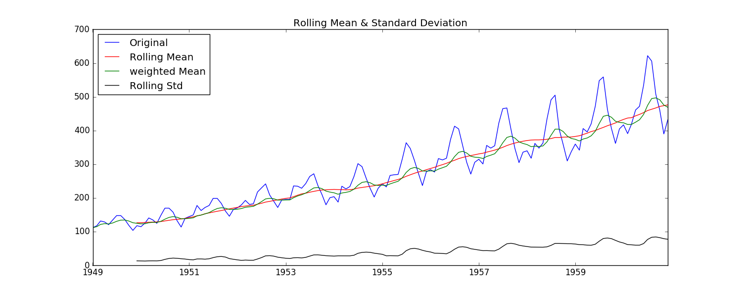
可以看到长期趋势和周期性的变动。
# estimating
ts_log = np.log(ts)
# plt.plot(ts_log)
# plt.show()
moving_avg = pd.rolling_mean(ts_log, 12)
# plt.plot(moving_avg)
# plt.plot(moving_avg,color='red')
# plt.show()
ts_log_moving_avg_diff = ts_log - moving_avg
# print ts_log_moving_avg_diff.head(12)
ts_log_moving_avg_diff.dropna(inplace=True)
test_stationarity(ts_log_moving_avg_diff)
plt.show()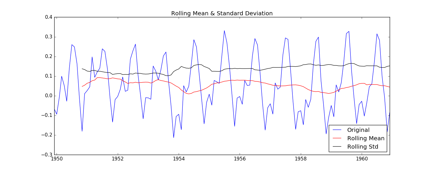
时间序列的差分d
# 差分differencing
ts_log_diff = ts_log.diff(1)
ts_log_diff.dropna(inplace=True)
test_stationarity(ts_log_diff)
plt.show()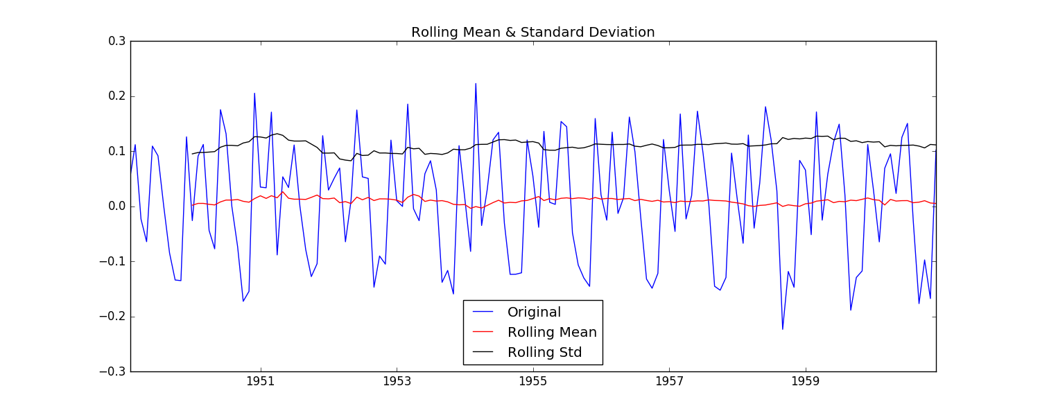
上图看出一阶差分大致已经具有周期性,不妨绘制二阶差分对比:
ts_log_diff1 = ts_log.diff(1)
ts_log_diff2 = ts_log.diff(2)
ts_log_diff1.plot()
ts_log_diff2.plot()
plt.show()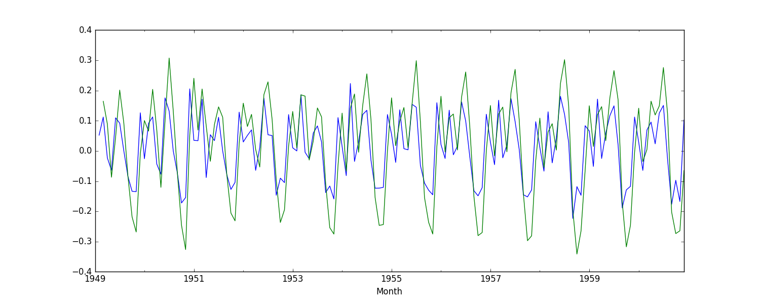
基本已经没有变化。所以使用一阶差分。
分解decomposing
# 分解decomposing
decomposition = seasonal_decompose(ts_log)

trend = decomposition.trend  # 趋势
seasonal = decomposition.seasonal  # 季节性
residual = decomposition.resid  # 剩余的

plt.subplot(411)
plt.plot(ts_log,label='Original')
plt.legend(loc='best')
plt.subplot(412)
plt.plot(trend,label='Trend')
plt.legend(loc='best')
plt.subplot(413)
plt.plot(seasonal,label='Seasonarity')
plt.legend(loc='best')
plt.subplot(414)
plt.plot(residual,label='Residual')
plt.legend(loc='best')
plt.tight_layout()
plt.show()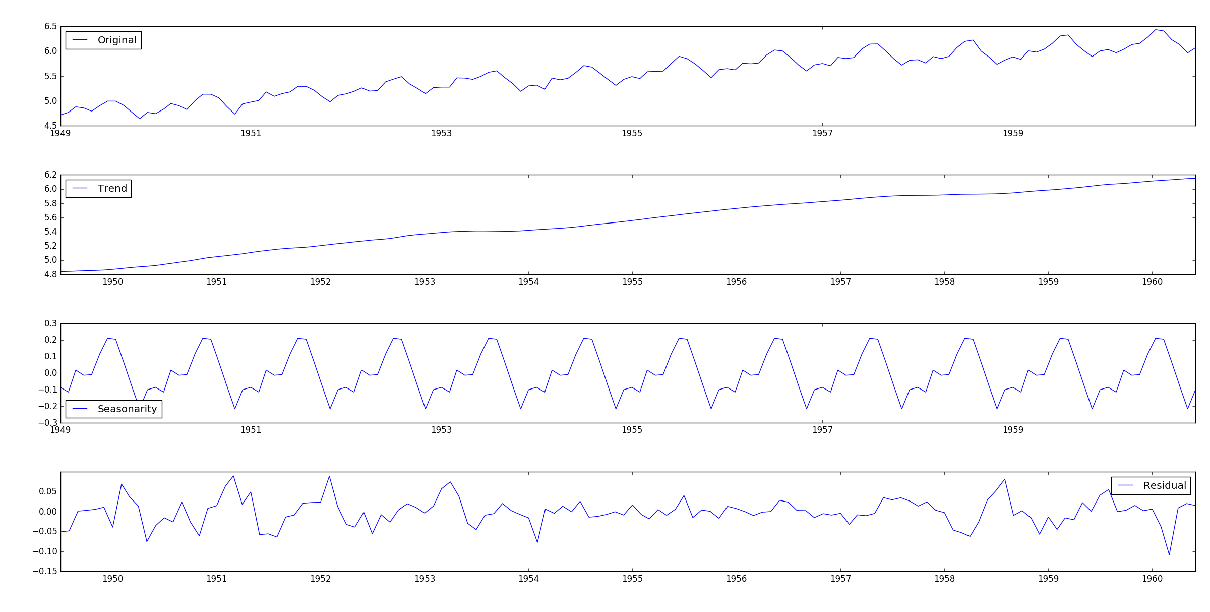
预测
确定参数
# 确定参数
lag_acf = acf(ts_log_diff, nlags=20)
lag_pacf = pacf(ts_log_diff, nlags=20, method='ols')
# q的获取:ACF图中曲线第一次穿过上置信区间.这里q取2
plt.subplot(121)
plt.plot(lag_acf)
plt.axhline(y=0, linestyle='--', color='gray')
plt.axhline(y=-1.96 / np.sqrt(len(ts_log_diff)), linestyle='--', color='gray')  # lowwer置信区间
plt.axhline(y=1.96 / np.sqrt(len(ts_log_diff)), linestyle='--', color='gray')  # upper置信区间
plt.title('Autocorrelation Function')
# p的获取:PACF图中曲线第一次穿过上置信区间.这里p取2
plt.subplot(122)
plt.plot(lag_pacf)
plt.axhline(y=0, linestyle='--', color='gray')
plt.axhline(y=-1.96 / np.sqrt(len(ts_log_diff)), linestyle='--', color='gray')
plt.axhline(y=1.96 / np.sqrt(len(ts_log_diff)), linestyle='--', color='gray')
plt.title('Partial Autocorrelation Function')
plt.tight_layout()
plt.show()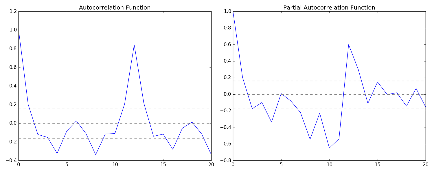
AR model
model = ARIMA(ts_log, order=(2, 1, 0))
result_AR = model.fit(disp=-1)
plt.plot(ts_log_diff)
plt.plot(result_AR.fittedvalues, color='red')
plt.title('AR model RSS:%.4f' % sum(result_AR.fittedvalues - ts_log_diff) ** 2)
plt.show()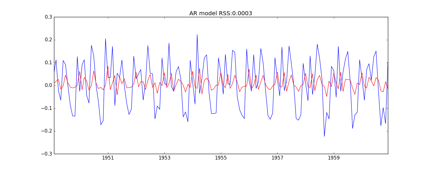
MA model
# MA model
model = ARIMA(ts_log, order=(0, 1, 2))
result_MA = model.fit(disp=-1)
plt.plot(ts_log_diff)
plt.plot(result_MA.fittedvalues, color='red')
plt.title('MA model RSS:%.4f' % sum(result_MA.fittedvalues - ts_log_diff) ** 2)
plt.show()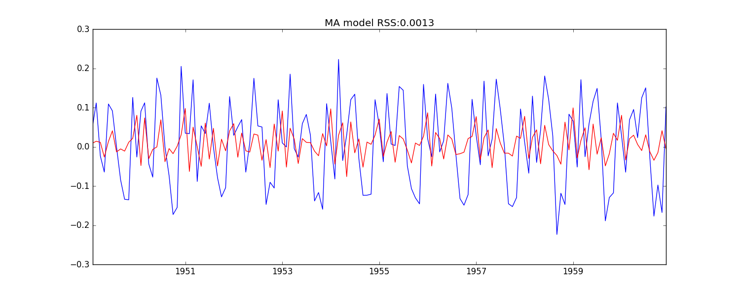
ARIMA model
# ARIMA 将两个结合起来  效果更好
model = ARIMA(ts_log, order=(2, 1, 2))
result_ARIMA = model.fit(disp=-1)
plt.plot(ts_log_diff)
plt.plot(result_ARIMA.fittedvalues, color='red')
plt.title('ARIMA RSS:%.4f' % sum(result_ARIMA.fittedvalues - ts_log_diff) ** 2)
plt.show()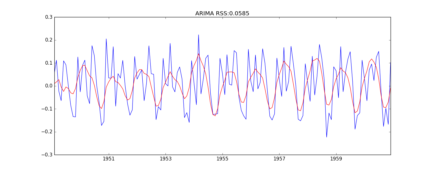
predictions_ARIMA
predictions_ARIMA_diff = pd.Series(result_ARIMA.fittedvalues, copy=True)
# print predictions_ARIMA_diff.head()#发现数据是没有第一行的,因为有1的延迟

predictions_ARIMA_diff_cumsum = predictions_ARIMA_diff.cumsum()
# print predictions_ARIMA_diff_cumsum.head()

predictions_ARIMA_log = pd.Series(ts_log.ix[0], index=ts_log.index)
predictions_ARIMA_log = predictions_ARIMA_log.add(predictions_ARIMA_diff_cumsum, fill_value=0)
# print predictions_ARIMA_log.head()

predictions_ARIMA = np.exp(predictions_ARIMA_log)
plt.plot(ts)
plt.plot(predictions_ARIMA)
plt.title('predictions_ARIMA RMSE: %.4f' % np.sqrt(sum((predictions_ARIMA - ts) ** 2) / len(ts)))
plt.show()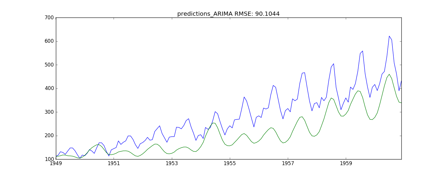


 3630
3630


 被折叠的 条评论
为什么被折叠?
被折叠的 条评论
为什么被折叠?
 到【灌水乐园】发言


