


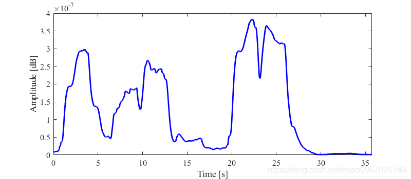
1.瞬时能量
信号瞬时能量定义为:
对于信号,在此信号上应用第 个帧窗口:
是窗长
是帧移
MATLAB 代码:
function En = energy(x,wintype,winamp,winlen)
%ENERGY   Short-time energy computation.
%   y = ENERGY(X,WINTYPE,WINAMP,WINLEN) computes the short-time enery of
%   the sequence X.
%
%   WINTYPE defines the window type. RECTWIN, HAMMING, HANNING, and
%   BLACKAMN are the possible choices. WINAMP sets the amplitude of the
%   window and the length of the window is WINLEN.


error(nargchk(1,4,nargin,'struct'));

% generate the window
win = (winamp*(window(str2func(wintype),winlen))).';

% enery calculation
x2 = x.^2;
En = winconv(x2,wintype,win,winlen);
结果:

2.过零率
信号中的高频段有高的过零率,低频段过零率较低。短时能量大的地方过零率小,短时能量小的地方过零率较大。
其中,
MATLAB源代码:
function zc = zerocross(x,wintype,winamp,winlen)
%ENERGY   Short-time energy computation.
%   y = ZEROCROSS(X,WINTYPE,WINAMP,WINLEN) computes the short-time enery of
%   the sequence X.
%
%   WINTYPE defines the window type. RECTWIN, HAMMING, HANNING, and
%   BLACKAMN are the possible choices. WINAMP sets the amplitude of the
%   window and the length of the window is WINLEN.


error(nargchk(1,4,nargin,'struct'));

% generate x[n] and x[n-1]
x1 = x;
x2 = [0, x(1:end-1)];

% generate the first difference
firstDiff = sgn(x1)-sgn(x2);

% magnitude only
absFirstDiff = abs(firstDiff);

% lowpass filtering with window
zc = winconv(absFirstDiff,wintype,winamp,winlen);
结果:

3.排列熵
PE分析一维时间序列,便于分析,考虑一个示例:
划分状态空间:将一维时间序列划分为重叠列向量的矩阵。 此分区使用两个超参数:
:嵌入时间延迟,它控制每个新列向量的元素之间的时间段数。默认值为
。
:嵌入尺寸,用于控制每个新列向量的长度。默认值为
。
用 和
,示例数据按以下方式划分:
每个列向量都有3个元素,因为嵌入维设置为3。此外,由于嵌入时间延迟设置为1,因此向量中每个元素之间只有一个时间段。为
维向量创建的列向量的数量为
。
示例数据的矩阵包含列向量 。
划分一维时间序列后,维向量映射到唯一的排列中,这些排列捕获数据的有序排列:
遵循上面的示例,总共有不同的可能排列(普通模式):
这些置换根据值在矢量中的顺序位置将值分配给每个分区矢量。 考虑示例的首3维向量
因为 ,此向量的置换是
。 因此,对于示例数据,置换矩阵为
如果输入向量包含两个或多个具有相同值的元素,则排名由它们在序列中的顺序确定。通过添加白噪声来打破平局,其中随机项的强度小于值之间的最小距离。
计算相对频率:可以通过计算在时间序列中找到置换的次数除以序列总数,来计算每个置换的相对频率。
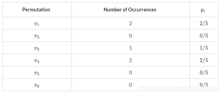
计算PE:最后,先前的概率用于计算时间序列阶数的PE,由下式给出:
继续上例,第3阶的PE为
PE中的PE值也可以标准化为
MATLAB代码:
function outdata = PE( indata, delay, order, windowSize )
% @brief PE efficiently [1] computes values of permutation entropy [2] in
% maximally overlapping sliding windows
%
% INPUT
%   - indata - considered time series
%   - delay - delay between points in ordinal patterns (delay = 1 means successive points)
%   - order - order of the ordinal patterns (order+1 - number of points in ordinal patterns)
%   - windowSize - size of sliding window
% OUTPUT
%   - outdata - values of normalised permutation entropy as defined in [2]
%
% REFERENCES
% [1] Unakafova, V.A., Keller, K., 2013. Efficiently measuring complexity
% on the basis of real-world data. Entropy, 15(10), 4392-4415.
% [2] Bandt C., Pompe B., 2002. Permutation entropy: a natural complexity
% measure for time series. Physical review letters, APS
%


 load( ['table' num2str( order ) '.mat'] ); % the precomputed table
 patternsTable = eval( ['table' num2str( order )] );
 nPoints    = numel( indata );              % length of the time series
 opOrder1   = order + 1;
 orderDelay = order*delay;
 nPatterns  = factorial( opOrder1 );   % amount of ordinal patterns
 patternsDistribution = zeros( 1, nPatterns ); % distribution of ordinal patterns
 outdata = zeros( 1, nPoints );        % values of permutation entropy
 inversionNumbers = zeros( 1, order ); % inversion numbers of ordinal pattern (i1,i2,...,id)
 prevOP = zeros( 1, delay );           % previous ordinal patterns for 1:opDelay
 ordinalPatternsInWindow = zeros( 1, windowSize ); % ordinal patterns in the window
 ancNum = nPatterns./factorial( 2:opOrder1 );  % ancillary numbers
 peTable( 1:windowSize ) = -( 1:windowSize ).*log( 1:windowSize  ); % table of precomputed values
 peTable( 2:windowSize ) = ( peTable( 2:windowSize ) - peTable( 1:windowSize - 1 ) )./windowSize;
 for iTau = 1:delay
     cnt = iTau;
     inversionNumbers( 1 ) = ( indata( orderDelay + iTau - delay ) >= indata( orderDelay + iTau ) );
     for j = 2:order
         inversionNumbers( j ) = sum( indata( ( order - j )*delay + iTau ) >= ...
           indata( ( opOrder1 - j )*delay + iTau:delay:orderDelay + iTau ) );
     end
     ordinalPatternsInWindow( cnt ) = sum( inversionNumbers.*ancNum ); % first ordinal patterns
     patternsDistribution( ordinalPatternsInWindow( cnt )+ 1 ) = ...
       patternsDistribution( ordinalPatternsInWindow( cnt ) + 1 ) + 1;
     for j = orderDelay + delay + iTau:delay:windowSize + orderDelay   % loop for the first window
         cnt = cnt + delay;
         posL = 1; % the position of the next point
         for i = j - orderDelay:delay:j - delay
             if( indata( i ) >= indata( j ) )
                 posL = posL + 1;
             end
         end
         ordinalPatternsInWindow( cnt ) = ...
           patternsTable( ordinalPatternsInWindow( cnt - delay )*opOrder1 + posL );
         patternsDistribution( ordinalPatternsInWindow( cnt ) + 1 ) = ...
           patternsDistribution( ordinalPatternsInWindow( cnt ) + 1 ) + 1;
     end
     prevOP( iTau ) = ordinalPatternsInWindow( cnt );
 end
 ordDistNorm = patternsDistribution/windowSize;
 tempSum = 0;
 for iPattern = 1:nPatterns
   if ( ordDistNorm( iPattern ) ~= 0 )
     tempSum = tempSum - ordDistNorm( iPattern )*log( ordDistNorm( iPattern ) );
   end
 end
 outdata( windowSize + delay*order ) = tempSum;

 iTau = mod( windowSize, delay ) + 1;   % current shift 1:delay
 patternPosition = 1;                   % position of the current pattern in the window
 for t = windowSize + delay*order + 1:nPoints % loop over all points
     posL = 1;                          % the position of the next point
     for j = t-orderDelay:delay:t-delay
         if( indata( j ) >= indata( t ) )
             posL = posL + 1;
         end
     end
     nNew = patternsTable( prevOP( iTau )*opOrder1 + posL ); % incoming ordinal pattern
     nOut = ordinalPatternsInWindow( patternPosition );      % outcoming ordinal pattern
     prevOP( iTau ) = nNew;
     ordinalPatternsInWindow( patternPosition ) = nNew;
     nNew = nNew + 1;
     nOut = nOut + 1;
     if ( nNew ~= nOut ) % update the distribution of ordinal patterns
         patternsDistribution( nNew ) = patternsDistribution( nNew ) + 1; % incoming ordinal pattern
         patternsDistribution( nOut ) = patternsDistribution( nOut ) - 1; % outcoming ordinal pattern
         outdata( t ) = outdata( t - 1 ) + ( peTable( patternsDistribution( nNew ) ) - ...
                                        peTable( patternsDistribution( nOut ) + 1  ) );
     else
         outdata( t ) = outdata( t - 1 );
     end
     iTau = iTau + 1;
     patternPosition = patternPosition + 1;
     if ( iTau > delay )
       iTau = 1;
     end
     if ( patternPosition > windowSize )
       patternPosition = 1;
     end
 end
 outdata = outdata( windowSize + delay*order:end )/log( factorial( order + 1 ) );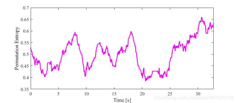


 3108
3108


 被折叠的 条评论
为什么被折叠?
被折叠的 条评论
为什么被折叠?
 到【灌水乐园】发言


