【吴恩达机器学习】逻辑回归 Python实现

课程笔记：https://blog.csdn.net/monochrome00/article/details/104109806

逻辑回归（Logistic Regression）

梯度下降版本

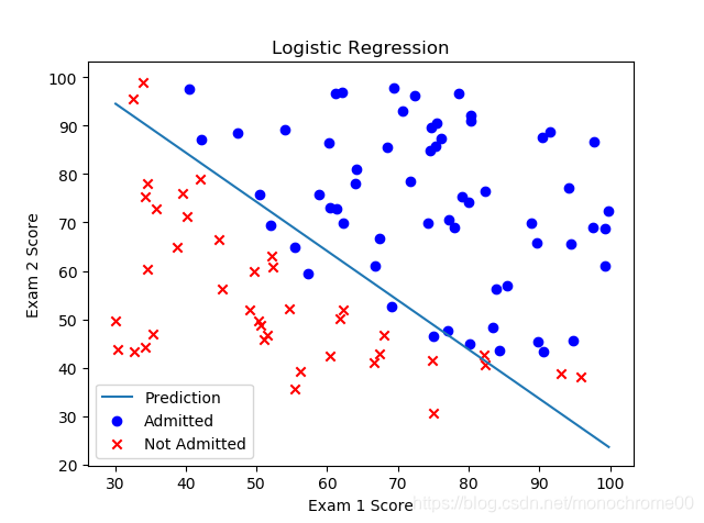
吴恩达课程给出来的数据因为是给优化跑的，普通的梯度下降跑不出来，除非初始值设$[-100,1,1]$这样的。

import numpy as np
import pandas as pd
import matplotlib.pyplot as plt


# 获取数据
def getData():
    path = "ex2data1.txt"
    returnData = pd.read_csv(path, header=None, names=['exam1', 'exam2', 'admitted'])
    return returnData


# sigmoid函数
def sigmoid(z):
    return 1 / (1 + np.exp(-z))


# 获取假设函数
def getHypothesis(X, theta):
    return sigmoid((theta @ X.T)).T


# 获取代价函数
def getCost(X, y, theta):
    h = getHypothesis(X, theta)
    return -np.mean(y * np.log(h.T) + (1 - y) * np.log(1 - h.T))


def gradientDescent(X, y):
    theta = np.asmatrix([[-100, 1, 1]])  # 按照X的列数设定theta的大小
    for i in range(0, epoch):
        theta = theta - alpha / len(y) * (getHypothesis(X, theta) - y).T * X
        now = getCost(X, y, theta)
    return theta


if __name__ == '__main__':
    data = getData()

    # 绘制样本点
    positive = data[data.admitted.isin(['1'])]
    negative = data[data.admitted.isin(['0'])]
    fig, ax = plt.subplots()
    ax.scatter(positive.exam1, positive.exam2, c='b', label='Admitted')
    ax.scatter(negative.exam1, negative.exam2, c='r', marker='x', label='Not Admitted')
    ax.set_xlabel("Exam 1 Score")
    ax.set_ylabel("Exam 2 Score")
    ax.set_title("Logistic Regression")
    plt.legend()

    # 分割输入和输出
    data.insert(0, 'x0', 1)  # 添加一列1
    col = data.shape[1]
    X = np.asmatrix(data.iloc[:, 0:col - 1])
    y = np.asmatrix(data.iloc[:, col - 1:col])

    epoch = 1000  # 迭代次数
    alpha = 0.001  # 学习速率
    finalTheta = gradientDescent(X, y)  # 梯度下降
    print(finalTheta)

    # 绘制预测图像
    x = np.linspace(data.exam1.min(), data.exam1.max(), 1000)  # 横坐标
    f = -finalTheta[0, 0] / finalTheta[0, 2] - finalTheta[0, 1] / finalTheta[0, 2] * x  # 直接计算出y坐标
    plt.plot(x, f, label='Prediction')  # 画出最后所得的模型
    plt.legend()
    plt.show()

最后的效果：

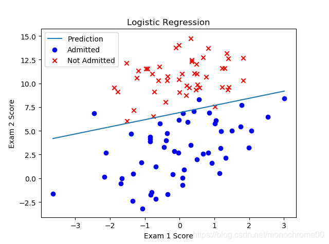
网上扒到一个好跑一点的，或者说就是让你跑初始值$[0,0,0]$的：https://blog.csdn.net/L_15156024189/article/details/85601302

-0.017612,14.053064,0
-1.395634,4.662541,1
-0.752157,6.538620,0
-1.322371,7.152853,0
0.423363,11.054677,0
0.406704,7.067335,1
0.667394,12.741452,0
-2.460150,6.866805,1
0.569411,9.548755,0
-0.026632,10.427743,0
0.850433,6.920334,1
1.347183,13.175500,0
1.176813,3.167020,1
-1.781871,9.097953,0
-0.566606,5.749003,1
0.931635,1.589505,1
-0.024205,6.151823,1
-0.036453,2.690988,1
-0.196949,0.444165,1
1.014459,5.754399,1
1.985298,3.230619,1
-1.693453,-0.557540,1
-0.576525,11.778922,0
-0.346811,-1.678730,1
-2.124484,2.672471,1
1.217916,9.597015,0
-0.733928,9.098687,0
-3.642001,-1.618087,1
0.315985,3.523953,1
1.416614,9.619232,0
-0.386323,3.989286,1
0.556921,8.294984,1
1.224863,11.587360,0
-1.347803,-2.406051,1
1.196604,4.951851,1
0.275221,9.543647,0
0.470575,9.332488,0
-1.889567,9.542662,0
-1.527893,12.150579,0
-1.185247,11.309318,0
-0.445678,3.297303,1
1.042222,6.105155,1
-0.618787,10.320986,0
1.152083,0.548467,1
0.828534,2.676045,1
-1.237728,10.549033,0
-0.683565,-2.166125,1
0.229456,5.921938,1
-0.959885,11.555336,0
0.492911,10.993324,0
0.184992,8.721488,0
-0.355715,10.325976,0
-0.397822,8.058397,0
0.824839,13.730343,0
1.507278,5.027866,1
0.099671,6.835839,1
-0.344008,10.717485,0
1.785928,7.718645,1
-0.918801,11.560217,0
-0.364009,4.747300,1
-0.841722,4.119083,1
0.490426,1.960539,1
-0.007194,9.075792,0
0.356107,12.447863,0
0.342578,12.281162,0
-0.810823,-1.466018,1
2.530777,6.476801,1
1.296683,11.607559,0
0.475487,12.040035,0
-0.783277,11.009725,0
0.074798,11.023650,0
-1.337472,0.468339,1
-0.102781,13.763651,0
-0.147324,2.874846,1
0.518389,9.887035,0
1.015399,7.571882,0
-1.658086,-0.027255,1
1.319944,2.171228,1
2.056216,5.019981,1
-0.851633,4.375691,1
-1.510047,6.061992,0
-1.076637,-3.181888,1
1.821096,10.283990,0
3.010150,8.401766,1
-1.099458,1.688274,1
-0.834872,-1.733869,1
-0.846637,3.849075,1
1.400102,12.628781,0
1.752842,5.468166,1
0.078557,0.059736,1
0.089392,-0.715300,1
1.825662,12.693808,0
0.197445,9.744638,0
0.126117,0.922311,1
-0.679797,1.220530,1
0.677983,2.556666,1
0.761349,10.693862,0
-2.168791,0.143632,1
1.388610,9.341997,0
0.317029,14.739025,0

这组数据好看很多，如果调整一下迭代次数，可以比较清楚的看到线条的变化。

---

高级优化算法

在练习中，一个称为“fminunc”的Octave函数是用来优化函数来计算成本和梯度参数。由于我们使用Python，我们可以用SciPy的“optimize”命名空间来做同样的事情。
这里我们使用的是高级优化算法，运行速度通常远远超过梯度下降。方便快捷。
只需传入cost函数，已经所求的变量theta，和梯度。cost函数定义变量时变量tehta要放在第一个，若cost函数只返回cost，则设置fprime=gradient。

# coding=gbk
import numpy as np
import pandas as pd
import matplotlib.pyplot as plt
import scipy.optimize as opt


# 获取数据
def getData():
    path = "ex2data1.txt"
    returnData = pd.read_csv(path, header=None, names=['exam1', 'exam2', 'admitted'])
    return returnData


# sigmoid函数
def sigmoid(z):
    return 1 / (1 + np.exp(-z))


# 获取假设函数
def getHypothesis(theta, X):
    return sigmoid(X @ theta)


# 获取代价函数
def getCost(theta, X, y):
    h = getHypothesis(theta, X)
    return -np.mean(y * np.log(h) + (1 - y) * np.log(1 - h))


# 梯度
def gradient(theta, X, y):
    return X.T @ (getHypothesis(theta, X) - y) / len(X)


# 根据theta和输入X来进行预测
def predict(theta, X):
    probability = getHypothesis(theta, X)
    return [1 if x >= 0.5 else 0 for x in probability]  # 返回值是一个list


# 得到模型预测精度
def getAccuracy(theta, X, y):
    predictions = predict(theta, X)
    correct = [1 if a == b else 0 for (a, b) in zip(predictions, y)]
    return sum(correct) / len(X)


if __name__ == '__main__':
    data = getData()
    # 绘制样本点
    positive = data[data.admitted.isin(['1'])]
    negative = data[data.admitted.isin(['0'])]
    fig, ax = plt.subplots()
    ax.scatter(positive.exam1, positive.exam2, c='b', label='Admitted')
    ax.scatter(negative.exam1, negative.exam2, c='r', marker='x', label='Not Admitted')
    ax.set_xlabel("Exam 1 Score")
    ax.set_ylabel("Exam 2 Score")
    ax.set_title("Advanced Optimization")

    # 分割输入和输出
    data.insert(0, 'x0', 1)  # 添加一列1
    X = data.iloc[:, :-1].values
    y = data.iloc[:, -1].values

    # 进行高级优化算法
    theta = np.zeros(X.shape[1])
    result = opt.fmin_tnc(func=getCost, x0=theta, fprime=gradient, args=(X, y))
    finalTheata = result[0]
    print(result)
    print(getCost(finalTheata, X, y))
    print(getAccuracy(theta, X, y))

    # 绘制预测图像
    x = np.linspace(data.exam1.min(), data.exam1.max(), 1000)  # 横坐标
    f = -finalTheata[0] / finalTheata[2] - finalTheata[1] / finalTheata[2] * x  # 直接计算出y坐标
    plt.plot(x, f, label='Prediction')  # 画出最后所得的模型
    plt.legend()
    plt.show()