


[python]bokeh学习总结——QuickStart
bokeh是python中一款基于网页的画图工具库,画出的图像以html格式保存。
一个简单的例子:
-
from bokeh.plotting
import figure, output_file, show
-
-
output_file(
"patch.html")
-
-
p = figure(plot_width=
400, plot_height=
400)
-
-
# add a patch renderer with an alpha an line width
-
p.patch([
1,
2,
3,
4,
5], [
6,
7,
8,
7,
3], alpha=
0.5, line_width=
2)
-
-
show(p)
画出图像后:

代码中有一行为
from bokeh.plotting import figure
figure是一个什么类型的数据?通过查看源代码,发现原来figure是一个函数,返回值为Figure类,Figure类以来自bokeh.models中的Plot类为父类,Figure类继承了Plot类中的各种属性。
Plotting with Basic Glyphs
Creating Figures
Scatter Markers
画出圆形可以使用circle()方法:
-
from bokeh.plotting
import figure, output_file, show
-
-
# output to static HTML file
-
output_file(
"line.html")
-
-
p = figure(plot_width=
400, plot_height=
400)
-
-
# add a circle renderer with a size, color, and alpha
-
p.circle([
1,
2,
3,
4,
5], [
6,
7,
2,
4,
5], size=
20, color=
"navy", alpha=
0.5)
-
-
# show the results
-
show(p)
得到的图形为:

同样的,如果要画出方形,可以使用square()方法,参数都是一样,将代码中的circle替换为square即可:
-
from bokeh.plotting
import figure, output_file, show
-
-
# output to static HTML file
-
output_file(
"square.html")
-
-
p = figure(plot_width=
400, plot_height=
400)
-
-
# add a square renderer with a size, color, and alpha
-
p.square([
1,
2,
3,
4,
5], [
6,
7,
2,
4,
5], size=
20, color=
"olive", alpha=
0.5)
-
-
# show the results
-
show(p)
画出的图形为:

还有许多其它图形函数,其参数也都是一样,x表示x轴的数据,y表示y轴的数据,size表示图形的大小。还有一些参数包含angle——表示角度的大小,radius——表示图形的半径。
详细使用方法见:
https://bokeh.pydata.org/en/latest/docs/reference/plotting.html#bokeh.plotting.figure.Figure.x
以annular_wedge()函数为例:
-
from bokeh.plotting
import figure, output_file, show
-
-
# output to static HTML file
-
output_file(
"square.html")
-
-
p = figure()
-
x = [
61,
62,
63,
64,
65]
-
y = [
66,
67,
68,
69,
70]
-
-
# add a square renderer with a size, color, and alpha
-
p.annular_wedge(x=x, y=y, inner_radius=
0.1, outer_radius=
0.3, start_angle=
0, end_angle=
5, direction=
'anticlock')
-
-
# show the results
-
show(p)

Line Glyphs
Single Lines
-
from bokeh.plotting
import figure, output_file, show
-
-
output_file(
"line.html")
-
-
p = figure(plot_width=
400, plot_height=
400)
-
-
# add a line renderer
-
p.line([
1,
2,
3,
4,
5], [
6,
7,
2,
4,
5], line_width=
2)
-
-
show(p)

Step Lines
-
from bokeh.plotting
import figure, output_file, show
-
-
output_file(
"line.html")
-
-
p = figure(plot_width=
400, plot_height=
400)
-
-
# add a steps renderer
-
p.step([
1,
2,
3,
4,
5], [
6,
7,
2,
4,
5], line_width=
2, mode=
"center")
-
-
show(p)

Multiple Lines
-
from bokeh.plotting
import figure, output_file, show
-
-
output_file(
"patch.html")
-
-
p = figure(plot_width=
400, plot_height=
400)
-
-
p.multi_line([[
1,
3,
2], [
3,
4,
6,
6]], [[
2,
1,
4], [
4,
7,
8,
5]],
-
color=[
"firebrick",
"navy"], alpha=[
0.8,
0.3], line_width=
4)
-
-
show(p)

需要注意的是,第一个list表示x轴的数据,[[1,3,2],[3,4,6,6]]中的两个list代表lines是分离的;第二个list表示y轴的数据。
Missing Points
NaN可以作为line()和multi_line()函数参数的一部分,用该值可以表示不连续点。若x=NaN,则对应的y值将被忽略。
-
from bokeh.plotting
import figure, output_file, show
-
-
output_file(
"line.html")
-
-
p = figure(plot_width=
400, plot_height=
400)
-
-
# add a line renderer with a NaN
-
nan = float(
'nan')
-
p.line([
1,
2,
3, nan,
3,
5], [
6,
7,
2,
4,
4,
5], line_width=
2)
-
-
show(p)

Bars and Rectangles
Rectangles
-
from bokeh.plotting
import figure, show, output_file
-
-
output_file(
'rectangles.html')
-
-
p = figure(plot_width=
400, plot_height=
400)
-
p.quad(top=[
2,
3,
4], bottom=[
1,
2,
3], left=[
1,
2,
3],
-
right=[
1.2,
2.5,
3.7], color=
"#B3DE69")
-
-
show(p)

还有一个例子:
-
from math
import pi
-
from bokeh.plotting
import figure, show, output_file
-
-
output_file(
'rectangles_rotated.html')
-
-
p = figure(plot_width=
400, plot_height=
400)
-
p.rect(x=[
1,
2,
3], y=[
1,
2,
3], width=
0.2, height=
40, color=
"#CAB2D6",
-
angle=pi/
3, height_units=
"screen")
-
-
show(p)

Bars
vertical bars:
-
from bokeh.plotting
import figure, show, output_file
-
-
output_file(
'vbar.html')
-
-
p = figure(plot_width=
400, plot_height=
400)
-
p.vbar(x=[
1,
2,
3], width=
0.5, bottom=
0,
-
top=[
1.2,
2.5,
3.7], color=
"firebrick")
-
-
show(p)

horizon bars:
-
from bokeh.plotting
import figure, show, output_file
-
-
output_file(
'hbar.html')
-
-
p = figure(plot_width=
400, plot_height=
400)
-
p.hbar(y=[
1,
2,
3], height=
0.5, left=
0,
-
right=[
1.2,
2.5,
3.7], color=
"navy")
-
-
show(p)

Hex Tiles
-
import numpy
as np
-
-
from bokeh.io
import output_file, show
-
from bokeh.plotting
import figure
-
from bokeh.util.hex
import axial_to_cartesian
-
-
output_file(
"hex_coords.py")
-
-
q = np.array([
0,
0,
0,
-1,
-1,
1,
1])
-
r = np.array([
0,
-1,
1,
0,
1,
-1,
0])
-
-
p = figure(plot_width=
400, plot_height=
400, toolbar_location=
None)
-
p.grid.visible =
False
-
-
p.hex_tile(q, r, size=
1, fill_color=[
"firebrick"]*
3 + [
"navy"]*
4,
-
line_color=
"white", alpha=
0.5)
-
-
x, y = axial_to_cartesian(q, r,
1,
"pointytop")
-
-
p.text(x, y, text=[
"(%d, %d)" % (q,r)
for (q, r)
in zip(q, r)],
-
text_baseline=
"middle", text_align=
"center")
-
-
show(p)

-
import numpy
as np
-
-
from bokeh.io
import output_file, show
-
from bokeh.plotting
import figure
-
from bokeh.transform
import linear_cmap
-
from bokeh.util.hex
import hexbin
-
-
n =
50000
-
x = np.random.standard_normal(n)
-
y = np.random.standard_normal(n)
-
-
bins = hexbin(x, y,
0.1)
-
-
p = figure(tools=
"wheel_zoom,reset", match_aspect=
True, background_fill_color=
'#440154')
-
p.grid.visible =
False
-
-
p.hex_tile(q=
"q", r=
"r", size=
0.1, line_color=
None, source=bins,
-
fill_color=linear_cmap(
'counts',
'Viridis256',
0, max(bins.counts)))
-
-
output_file(
"hex_tile.html")
-
-
show(p)

Patch Glyphs
Single Patches
-
from bokeh.plotting
import figure, output_file, show
-
-
output_file(
"patch.html")
-
-
p = figure(plot_width=
400, plot_height=
400)
-
-
# add a patch renderer with an alpha an line width
-
p.patch([
1,
2,
3,
4,
5], [
6,
7,
8,
7,
3], alpha=
0.5, line_width=
2)
-
-
show(p)

Multiple Patches
-
from bokeh.plotting
import figure, output_file, show
-
-
output_file(
"patch.html")
-
-
p = figure(plot_width=
400, plot_height=
400)
-
-
p.patches([[
1,
3,
2], [
3,
4,
6,
6]], [[
2,
1,
4], [
4,
7,
8,
5]],
-
color=[
"firebrick",
"navy"], alpha=[
0.8,
0.3], line_width=
2)
-
-
show(p)

Missing Points
-
from bokeh.plotting
import figure, output_file, show
-
-
output_file(
"patch.html")
-
-
p = figure(plot_width=
400, plot_height=
400)
-
-
# add a patch renderer with a NaN value
-
nan = float(
'nan')
-
p.patch([
1,
2,
3, nan,
4,
5,
6], [
6,
7,
5, nan,
7,
3,
6], alpha=
0.5, line_width=
2)
-
-
show(p)

Ovals and Ellipses
-
from math
import pi
-
from bokeh.plotting
import figure, show, output_file
-
-
output_file(
'ovals.html')
-
-
p = figure(plot_width=
400, plot_height=
400)
-
p.oval(x=[
1,
2,
3], y=[
1,
2,
3], width=
0.2, height=
40, color=
"#CAB2D6",
-
angle=pi/
3, height_units=
"screen")
-
-
show(p)

-
from math
import pi
-
from bokeh.plotting
import figure, show, output_file
-
-
output_file(
'ellipses.html')
-
-
p = figure(plot_width=
400, plot_height=
400)
-
p.ellipse(x=[
1,
2,
3], y=[
1,
2,
3], width=[
0.2,
0.3,
0.1], height=
0.3,
-
angle=pi/
3, color=
"#CAB2D6")
-
-
show(p)

Segments and Rays
Sometimes it is useful to be able to draw many individual line segments at once. Bokeh provides the segment() and ray() glyph methods to render these.
-
from bokeh.plotting
import figure, show
-
-
p = figure(plot_width=
400, plot_height=
400)
-
p.segment(x0=[
1,
2,
3], y0=[
1,
2,
3], x1=[
1.2,
2.4,
3.1],
-
y1=[
1.2,
2.5,
3.7], color=
"#F4A582", line_width=
3)
-
-
show(p)

The ray() function accepts start points x, y with a length (in screen units) and an angle. The default angle_units are "rad" but can also be changed to "deg". To have an “infinite” ray, that always extends to the edge of the plot, specify 0 for the length:
-
from bokeh.plotting
import figure, show
-
-
p = figure(plot_width=
400, plot_height=
400)
-
p.ray(x=[
1,
2,
3], y=[
1,
2,
3], length=
45, angle=[
30,
45,
60],
-
angle_units=
"deg", color=
"#FB8072", line_width=
2)
-
-
show(p)

Wedges and Arcs
-
from bokeh.plotting
import figure, show
-
-
p = figure(plot_width=
400, plot_height=
400)
-
p.arc(x=[
1,
2,
3], y=[
1,
2,
3], radius=
0.1, start_angle=
0.4, end_angle=
4.8, color=
"navy")
-
-
show(p)

-
from bokeh.plotting
import figure, show
-
-
p = figure(plot_width=
400, plot_height=
400)
-
p.wedge(x=[
1,
2,
3], y=[
1,
2,
3], radius=
0.2, start_angle=
0.4, end_angle=
4.8,
-
color=
"firebrick", alpha=
0.6, direction=
"clock")
-
-
show(p)

-
from bokeh.plotting
import figure, show
-
-
p = figure(plot_width=
400, plot_height=
400)
-
p.annular_wedge(x=[
1,
2,
3], y=[
1,
2,
3], inner_radius=
0.1, outer_radius=
0.25,
-
start_angle=
0.4, end_angle=
4.8, color=
"green", alpha=
0.6)
-
-
show(p)

-
from bokeh.plotting
import figure, show
-
-
p = figure(plot_width=
400, plot_height=
400)
-
p.annulus(x=[
1,
2,
3], y=[
1,
2,
3], inner_radius=
0.1, outer_radius=
0.25,
-
color=
"orange", alpha=
0.6)
-
-
show(p)

Combining Multiple Glyphs
-
from bokeh.plotting
import figure, output_file, show
-
-
x = [
1,
2,
3,
4,
5]
-
y = [
6,
7,
8,
7,
3]
-
-
output_file(
"multiple.html")
-
-
p = figure(plot_width=
400, plot_height=
400)
-
-
# add both a line and circles on the same plot
-
p.line(x, y, line_width=
2)
-
p.circle(x, y, fill_color=
"white", size=
8)
-
-
show(p)

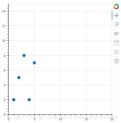
Setting Ranges
两种方法设置range:
1.可以通过从bokeh.models中导入Range1d(x,y)对象来实现:
By default, Bokeh will attempt to automatically set the data bounds of plots to fit snugly around the data. Sometimes you may need to set a plot’s range explicitly. This can be accomplished by setting the x_range or y_range properties using a Range1dobject that gives the start and end points of the range you want:
p.x_range = Range1d(0, 100)
2.在figure()里直接调用x_range()和y_range():
As a convenience, the figure() function can also accept tuples of (start, end) as values for the x_range or y_range parameters.
看一个例子:
-
from bokeh.plotting
import figure, output_file, show
-
from bokeh.models
import Range1d
-
-
output_file(
"title.html")
-
-
# create a new plot with a range set with a tuple
-
p = figure(plot_width=
400, plot_height=
400, x_range=(
0,
20))
-
-
# set a range using a Range1d
-
p.y_range = Range1d(
0,
15)
-
-
p.circle([
1,
2,
3,
4,
5], [
2,
5,
8,
2,
7], size=
10)
-
-
show(p)
Specifying Axis Types
Categorical Axes
上面的所有例子中,x和y轴都是数字,有些时候希望坐标轴显示的是字符,可以使用如下方法:
-
from bokeh.plotting
import figure, output_file, show
-
-
factors = [
"a",
"b",
"c",
"d",
"e",
"f",
"g",
"h"]
-
x = [
50,
40,
65,
10,
25,
37,
80,
60]
-
-
output_file(
"categorical.html")
-
-
p = figure(y_range=factors)
-
-
p.circle(x, factors, size=
15, fill_color=
"orange", line_color=
"green", line_width=
3)
-
-
show(p)
此时,y轴是factors:

Log Scale Axes
-
from bokeh.plotting
import figure, output_file, show
-
-
x = [
0.1,
0.5,
1.0,
1.5,
2.0,
2.5,
3.0]
-
y = [
10**xx
for xx
in x]
-
-
output_file(
"log.html")
-
-
# create a new plot with a log axis type
-
p = figure(plot_width=
400, plot_height=
400, y_axis_type=
"log")
-
-
p.line(x, y, line_width=
2)
-
p.circle(x, y, fill_color=
"white", size=
8)
-
-
show(p)

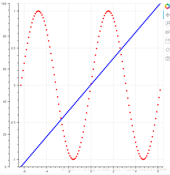
Twin Axes
-
from numpy
import pi, arange, sin, linspace
-
-
from bokeh.plotting
import output_file, figure, show
-
from bokeh.models
import LinearAxis, Range1d
-
-
x = arange(
-2*pi,
2*pi,
0.1)
-
y = sin(x)
-
y2 = linspace(
0,
100, len(y))
-
-
output_file(
"twin_axis.html")
-
-
p = figure(x_range=(
-6.5,
6.5), y_range=(
-1.1,
1.1))
-
-
p.circle(x, y, color=
"red")
-
-
p.extra_y_ranges = {
"foo": Range1d(start=
0, end=
100)}
-
p.circle(x, y2, color=
"blue", y_range_name=
"foo")
-
p.add_layout(LinearAxis(y_range_name=
"foo"),
'left')
-
-
show(p)


 743
743

 被折叠的 条评论
为什么被折叠?
被折叠的 条评论
为什么被折叠?
 到【灌水乐园】发言


