基于OSQP的二次规划

1. 问题建模

  假设已知一条参考轨迹为$r_0,r_1,...,r_i,...,r_n$，这条轨迹可以任意生成，因为其中可能有直角拐点或者锐角拐点，机器人无法直接沿着该轨迹移动。因此，需要生成一条满足机器人运动学约束、尽可能平滑的实际可行的轨迹$x_0,x_1,...,x_i,...x_n$，这也是我们需要优化的变量，这里轨迹 { r i } \{r_i\} {ri​}和 { x i } \{x_i\} {xi​}具有相同的长度。由此建立下面的代价函数（$\text{cost function}$ ）：

$$\mathcal{J}=w_x\sum _{i=0}^{n-1}(x_i-r_i{)}^2+w_{x^{\prime }}\sum _{i=0}^{n-1}(x_i^{\prime }{)}^2+w_{x^{\prime \prime }}\sum _{i=0}^{n-1}(x_i^{\prime \prime }{)}^2+w_{x^{\prime \prime \prime }}\sum _{i=0}^{n-1}(x_i^{\prime \prime \prime }{)}^2$$

• $w_x{\sum }_{i=0}^{n-1}(x_i-r_i{)}^2$：最小化生成轨迹和参考轨迹之间的距离，也即让生成轨迹尽可能的沿着参考轨迹，其中$w_x$为权重。
• $w_{x^{\prime }}{\sum }_{i=0}^{n-1}(x_i^{\prime }{)}^2$：最小化轨迹的一阶导，其中$w_x^{\prime }$为权重。通俗点讲， { x } \{x\} {x}为轨迹时， { x ′ } \{x'\} {x′}为速度，这一项的目的是最小化速度。就像开车的时候，沿直线运动轨迹最短，能耗最小，乱打方向盘会让轨迹扭曲，加大能耗和移动时间。
• $w_x{\sum }_{i=0}^{n-1}(x_i-r_i{)}^2$：最小化轨迹的二阶导，其中$w_x^{\prime \prime }$为权重。通俗点讲，就是最小化加速度。
• $w_x{\sum }_{i=0}^{n-1}(x_i-r_i{)}^2$：最小化轨迹的三阶导，其中$w_x^{\prime \prime \prime }$为权重。通俗点讲，就是最小化加加速度（专业术语应该叫$\textbf{Jerk}）。

2. QP问题

  常见格式如下：
$$\begin{array}{r}min\frac{1}{2}{x}^T\mathcal{P}x+qx\\ l\le Ax\le u\end{array}$$

  其中$P$是一个$nxn$矩阵，$x$为$n$维向量，$q$为$mxn$的矩阵。

  为什么要转换成QP格式？

  因为QP问题一定是可求解的，而且目前各种求解器都支持求解QP问题，速度相对于非线性优化问题快了很多很多很多。

3. 格式转换

  下面将我们的问题转换成QP格式，主要就是构建$\mathcal{P}$矩阵和$q$矩阵，下面的内容主要参考这篇文章规划控制:Piecewise Jerk Path Optimizer的python实现。这里将参考文章种的一维拓展到二维，即 x = { x 0 , x 1 , . . . , x n } x=\{x_0,x_1, ..., x_n\} x={x0​,x1​,...,xn​}，其中每个状态 x i = { p x i , p y i , v x i , v y i , a x i , a y i } x_i=\{p_{xi},p_{yi},v_{xi},v_{yi},a_{xi},a_{yi}\} xi​={pxi​,pyi​,vxi​,vyi​,axi​,ayi​}，分别对应在$xy$轴上的位置$p_x$或$p_y$、速度$v_x$或$v_y$和加速度$a_x$或$a_y$。

  为了简化QP问题的规模，这里假设优化变量$x$包含$n$个状态（分别对应参考轨迹$r$的长度），且满足如下关系

• $x_i^{\prime }=\frac{x_{i+1}-x_i}{\Delta t}$
• $x_i^{\prime \prime }=\frac{x_{i+1}^{\prime }-x_i^{\prime }}{\Delta t}$
• $x_i^{\prime \prime \prime }=\frac{x_{i+1}^{\prime \prime }-x_i^{\prime \prime }}{\Delta t}$

  将上面最后一个公式带入代价函数$\mathcal{J}$中，并将其展开可得：
$$\mathcal{J}=w_x\sum _{i=0}^{n-1}[(x_i{)}^2+(r_i{)}^2-2x_i{r}_i]+w_{x^{\prime }}\sum _{i=0}^{n-1}(x_i^{\prime }{)}^2+w_{x^{\prime \prime }}\sum _{i=0}^{n-1}(x_i^{\prime \prime }{)}^2+\frac{w_{x^{\prime \prime \prime }}}{\Delta s^2}\sum _{i=0}^{n-2}[(x_{i+1}^{\prime \prime }{)}^2+(x_i^{\prime \prime }{)}^2-2x_{i+1}^{\prime \prime }{x}_i^{\prime \prime }]$$

去掉其中的常数项（和优化变量$x$无关的项）可得：

$$\mathcal{J}=w_x\sum _{i=0}^{n-1}[(x_i{)}^2-2x_i{r}_i]+w_{x^{\prime }}\sum _{i=0}^{n-1}(x_i^{\prime }{)}^2+(w_{x^{\prime \prime }}+\frac{2w_{x^{\prime \prime \prime }}}{\Delta s^2})\sum _{i=0}^{n-1}(x_i^{\prime \prime }{)}^2-\frac{w_{x^{\prime \prime \prime }}}{\Delta s^2}(x_0^{\prime \prime }+x_{n-1}^{\prime \prime })-\frac{2w_{x^{\prime \prime \prime }}}{\Delta s^2}\sum _{i=0}^{n-2}(x_{i+1}^{\prime \prime }{x}_i^{\prime \prime })$$

其中
$x=\left[\begin{array}{c}{x}_0\\ x_1\\ ⋮\\ x_{n-1}\\ x_0^{\prime }\\ x_1^{\prime }\\ ⋮\\ x_{n-1}^{\prime }\\ x_0^{\prime \prime }\\ x_1^{\prime \prime }\\ ⋮\\ x_{n-1}^{\prime \prime }\end{array}\right]=\left[\begin{array}{c}{p}_{x_0}\\ x_{x_1}\\ ⋮\\ p_{x_{n-1}}\\ p_{y_0}\\ p_{y_1}\\ ⋮\\ p_{y_n-1}\\ v_{x_0}\\ v_{x_1}\\ ⋮\\ v_{x_{n-1}}\\ v_{y_0}\\ v_{y_1}\\ ⋮\\ v_{y_{n-1}}\\ a_{x_0}\\ a_{x_1}\\ ⋮\\ a_{x_{n-1}}\\ a_{y_0}\\ a_{y_1}\\ ⋮\\ a_{y_{n-1}}\end{array}\right]\in R^{6n\times 1}$

构建$P$、$q$矩阵

$P_p=\left[\begin{array}{cccc}{w}_x& 0& \dots & 0\\ 0& w_x& \dots & 0\\ ⋮& ⋮& \ddots & ⋮\\ 0& 0& \dots & w_x\end{array}\right]\in R^{n\times n}，P_v=\left[\begin{array}{cccc}{w}_{x^{\prime }}& 0& \dots & 0\\ 0& w_{x^{\prime }}& \dots & 0\\ ⋮& ⋮& \ddots & ⋮\\ 0& 0& \dots & w_{x^{\prime }}\end{array}\right]\in R^{n\times n}$

$P_a=\left[\begin{array}{ccccc}{w}_{x^{\prime \prime }}+\frac{w_{x^{\prime \prime \prime }}}{\Delta s^2}& 0& \dots & 0& 0\\ -\frac{2w_{x^{\prime \prime \prime }}}{\Delta s^2}& w_{x^{\prime \prime }}+\frac{2w_{x^{\prime \prime \prime }}}{\Delta s^2}& \dots & 0& 0\\ ⋮& ⋮& \ddots & ⋮& ⋮\\ 0& 0& \dots & w_{x^{\prime \prime }}+\frac{2w_{x^{\prime \prime \prime }}}{\Delta s^2}& 0\\ 0& 0& \dots & -\frac{2w_{x^{\prime \prime \prime }}}{\Delta s^2}& w_{x^{\prime \prime }}+\frac{w_{x^{\prime \prime \prime }}}{\Delta s^2}\end{array}\right]\in R^{n\times n}$

$P=\left[\begin{array}{cccccc}{P}_p& & & & & \\ & P_p& & & & \\ & & P_v& & & \\ & & & P_v& & \\ & & & & P_a& \\ & & & & & P_a\end{array}\right]\in R^{6n\times 6n}$

$q=-\left[\begin{array}{c}{w}_x{p}_{x_0}\\ w_x{x}_{x_1}\\ ⋮\\ w_x{p}_{x_{n-1}}\\ w_x{p}_{y_0}\\ w_x{p}_{y_1}\\ ⋮\\ w_x{p}_{y_n-1}\\ w_{x^{\prime }}{v}_{x_0}\\ w_{x^{\prime }}{v}_{x_1}\\ ⋮\\ w_{x^{\prime }}{v}_{x_{n-1}}\\ w_{x^{\prime }}{v}_{y_0}\\ w_{x^{\prime }}{v}_{y_1}\\ ⋮\\ w_{x^{\prime }}{v}_{y_{n-1}}\\ w_{x^{\prime \prime }}{a}_{x_0}\\ w_{x^{\prime \prime }}{a}_{x_1}\\ ⋮\\ w_{x^{\prime \prime }}{a}_{x_{n-1}}\\ w_{x^{\prime \prime }}{a}_{y_0}\\ w_{x^{\prime \prime }}{a}_{y_1}\\ ⋮\\ w_{x^{\prime \prime }}{a}_{y_{n-1}}\end{array}\right]\in R^{1\times 6n}$

等式约束

  为了让生成的轨迹满足机器人的移动状态，需要将机器人的运动模型转换成对应的等式约束，即$l=Ax=u$。这里考虑如下运动模型：
$$\begin{array}{r}{x}_{i+1}=x_i+x_i^{\prime }\Delta t\\ x_{i+1}^{\prime }=x_i^{\prime }+x_i^{\prime \prime }\Delta t\\ x_{i+1}^{\prime \prime }=x_i^{\prime \prime }+x_i^{\prime \prime \prime }\Delta t\end{array}$$

转换成对应矩阵形式，此处以2维空间为例，即 x = { x 0 , x 1 , . . . , x n } x=\{x_0,x_1, ..., x_n\} x={x0​,x1​,...,xn​}，其中每个状态 x i = { p x i , p y i , v x i , v y i , a x i , a y i } x_i=\{p_{xi},p_{yi},v_{xi},v_{yi},a_{xi},a_{yi}\} xi​={pxi​,pyi​,vxi​,vyi​,axi​,ayi​}，分别对应在$xy$轴上的位置$p_x$或$p_y$、速度$v_x$或$v_y$和加速度$a_x$或$a_y$。

$A_I=\left[\begin{array}{ccccc}1& -1& 0& \dots & 0\\ 0& 1& -1& \dots & 0\\ ⋮& ⋮& \ddots & \ddots & ⋮\\ 0& 0& \dots & 1& -1\end{array}\right]\in R^{(n-1)\times n}$，

$A_t=\left[\begin{array}{ccccc}\Delta t& 0& 0& \dots & 0\\ 0& \Delta t& 0& \dots & 0\\ ⋮& ⋮& \ddots & \ddots & ⋮\\ 0& 0& \dots & \Delta t& 0\end{array}\right]\in R^{(n-1)\times n}$，

$A_z=\left[\begin{array}{ccccc}0& 0& 0& \dots & 0\\ 0& 0& 0& \dots & 0\\ ⋮& ⋮& \ddots & \ddots & ⋮\\ 0& 0& \dots & 0& 0\end{array}\right]\in R^{(n-1)\times n}$，

$A_{eq}=\left[\begin{array}{cccccc}{A}_I& A_z& A_t& A_z& A_z& A_z\\ A_z& A_I& A_z& A_t& A_z& A_z\end{array}\right]\in R^{(2n-2)\times 6n}$

$l_{eq}=u_{eq}=\left[\begin{array}{c}0\\ 0\\ ⋮\\ 0\end{array}\right]\in R^{6n\times 1}$

4. 使用OSQP求解问题

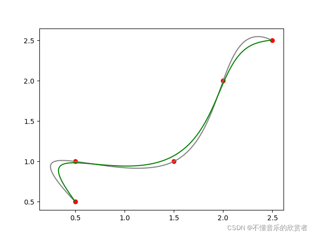
  效果如下，红色点是设置的路径点，灰色是b样条拟合的路径，绿色是优化的结果。

  直接上代码

import osqp
import numpy as np
import time
from scipy.interpolate import *
from scipy import sparse
import matplotlib.pyplot as plt


class PathOptimizer:
    def __init__(self, points, ts, acc, d='2d'):
        self.ctrl_points = points
        self.ctrl_ts = ts
        self.acc_max = acc
        self.dimension = d

        # 时间分配
        self.seg_length = self.acc_max * self.ctrl_ts * self.ctrl_ts
        self.total_length = 0
        for i in range(self.ctrl_points.shape[0] - 1):
            self.total_length += np.linalg.norm(self.ctrl_points[i + 1, :] - self.ctrl_points[i, :])
        self.total_time = self.total_length/self.seg_length * self.ctrl_ts * 1.2

        # 生成控制点B样条函数
        time_list = np.linspace(0, self.total_time, self.ctrl_points.shape[0])
        self.px_spline = InterpolatedUnivariateSpline(time_list, self.ctrl_points[:, 0])
        self.py_spline = InterpolatedUnivariateSpline(time_list, self.ctrl_points[:, 1])

        # 对B样条优化参考轨迹进行均匀采样
        self.seg_time_list = np.arange(0, self.total_time, self.ctrl_ts)
        self.px = self.px_spline(self.seg_time_list)
        self.py = self.py_spline(self.seg_time_list)

        # 优化问题权重参数
        self.weight_pos = 5
        self.weight_vel = 1
        self.weight_acc = 1
        self.weight_jerk = 0.1

        start_time = time.perf_counter()
        self.smooth_path = self.osqpSmooth()
        print('OSQP in ' + self.dimension + ' Cost time: ' + str(time.perf_counter() - start_time))
        pass

    def osqpSmooth(self):
        px0, py0 = self.px, self.py
        vx0 = vy0 = vz0 = np.zeros(self.px.shape)
        ax0 = ay0 = az0 = np.zeros(self.px.shape)

        # x(0), x(1), ..., x(n - 1), x'(0), x'(1), ..., x'(n - 1), x"(0), x"(1), ..., x"(n - 1)
        x0_total = np.hstack((px0, py0, vx0, vy0, ax0, ay0))


        n = int(x0_total.shape[0] / 3)   # 每种级别状态有几个变量,即x共n个，x'共n个，x"也是n个
        Q_x = self.weight_pos * np.eye(n)
        Q_dx = self.weight_vel * np.eye(n)
        Q_zeros = np.zeros((n, n))
        w_ddl = self.weight_acc
        w_dddl = self.weight_jerk

        if n % 2 != 0:
            print('x0 input error.')
            return
        n_part = int(n/2)   # 每部分有n_part个数据,即x_x(0), x_x(1), ..., x_x(n-1), x_y(0), x_y(1), ..., x_y(n-1), ...

        Q_ddx_part = (w_ddl + 2 * w_dddl / self.ctrl_ts / self.ctrl_ts) * np.eye(n_part) \
                     - 2 * w_dddl / self.ctrl_ts / self.ctrl_ts * np.eye(n_part, k=-1)
        Q_ddx_part[0][0] = w_ddl + w_dddl / self.ctrl_ts / self.ctrl_ts
        Q_ddx_part[n_part-1][n_part-1] = w_ddl + w_dddl / self.ctrl_ts / self.ctrl_ts

        np_zeros = np.zeros(Q_ddx_part.shape)
        Q_ddx_l = np.vstack((Q_ddx_part, np_zeros))
        Q_ddx_r = np.vstack((np_zeros, Q_ddx_part))
        Q_ddx = np.hstack((Q_ddx_l, Q_ddx_r))


        Q_total = sparse.csc_matrix(np.block([[Q_x, Q_zeros, Q_zeros],
                                              [Q_zeros, Q_dx, Q_zeros],
                                              [Q_zeros, Q_zeros, Q_ddx]
                                              ]))

        p_total = - x0_total
        p_total[:n] = self.weight_pos * p_total[:n]

        # 动力学模型，所以是等式约束
        # x(i+1) = x(i) + x'(i)△t
        # x'(i+1) = x'(i) + x"(i)△t
        AI_part = np.eye(n_part-1, n_part) - np.eye(n_part-1, n_part, k=1)  # 计算同阶变量之间插值 (n-1) x n维
        AT_part = self.ctrl_ts * np.eye(n_part-1, n_part)   # 时间矩阵 (n-1) x n维
        AZ_part = np.zeros([n_part-1, n_part])  # 全0矩阵 (n-1) x n维

        # 起点为第一个点
        A_init = np.zeros([4, x0_total.shape[0]])
        A_init[0, 0] = A_init[1, n_part] = 1
        A_init[2, n_part-1] = A_init[3, 2*n_part-1] = 1

        A_l_init = A_u_init = np.array([x0_total[0], x0_total[n_part],
                                        x0_total[n_part-1], x0_total[2*n_part-1]])

        A_eq = sparse.csc_matrix(np.block([
            [A_init],
            [AI_part, AZ_part, AT_part, AZ_part, AZ_part, AZ_part],
            [AZ_part, AI_part, AZ_part, AT_part, AZ_part, AZ_part],
            [AZ_part, AZ_part, AI_part, AZ_part, AT_part, AZ_part],
            [AZ_part, AZ_part, AZ_part, AI_part, AZ_part, AT_part]
        ]))
        A_leq = A_ueq = np.zeros(A_eq.shape[0])
        A_leq[:4] = A_ueq[:4] = A_l_init


        # Create an OSQP object
        prob = osqp.OSQP()
        prob.setup(Q_total, p_total, A_eq, A_leq, A_ueq, alpha=1.0)
        res = prob.solve()

        return res.x[:]


class PathGenerator:
    def __init__(self):
        self.ctrl_points = np.array([[0.5, 0.5],
                                     [0.5, 1],
                                     [1.5, 1.],
                                     [2., 2.],
                                     [2.5, 2.5]])

        self.ctrl_ts = 0.1  # 控制时间s
        self.acc_max = 2    # 米/秒

        self.ref_path = PathOptimizer(self.ctrl_points, self.ctrl_ts, self.acc_max)


if __name__ == '__main__':
    pg = PathGenerator()

    fig = plt.figure()

    ax = plt.axes()
    ax.scatter(pg.ctrl_points[:, 0], pg.ctrl_points[:, 1], color='red')
    ax.plot(pg.ref_path.px, pg.ref_path.py, color='gray')

    seg_num = pg.ref_path.px.shape[0]
    ax.plot(pg.ref_path.smooth_path[:seg_num], pg.ref_path.smooth_path[seg_num:2*seg_num], color='green')

    plt.show()