吴恩达cs229|编程作业第七周（Python）

最新推荐文章于 2023-03-08 19:19:39 发布

NotFound1911

最新推荐文章于 2023-03-08 19:19:39 发布

阅读量873

点赞数 1

分类专栏：自学

本文链接：https://blog.csdn.net/qq_24739717/article/details/88791760

版权

自学专栏收录该内容

78 篇文章 17 订阅

订阅专栏

练习七：k均值聚类与主成分分析

1.包含的文件。

2.k均值聚类。

3.（PCA）主成成分分析。

1.包含的文件。

文件名	含义
ex7.py	K-means实验
ex7_pca.py	PCA实验
ex7data1.mat	PCA实验数据集
ex7data2.mat	K-means实验数据集
ex7faces.mat	人脸数据集
bird_small.png	示例图片（鸟）
displayData.py	数据可视化
runkMeans.py	K-means算法
featureNormalize.py	特征归一化
projectData.py	原始数据从高维空间映射到低维空间
recoverData.py	将压缩数据恢复到原始数据
findClosestCentroids.py	找到最近的簇
computeCentroids.py	更新聚类中心
kMeansInitCentroids.py	初始化k-means的聚类中心
pca.py	PCA算法

注：红色部分需要自己填写。

2.K均值聚类

导入需要的包以及初始化：

import matplotlib.pyplot as plt
import numpy as np
import scipy.io as scio
from skimage import io
from skimage import img_as_float

import runkMeans as km
import findClosestCentroids as fc
import computeCentroids as cc
import kMeansInitCentroids as kmic

plt.ion()
np.set_printoptions(formatter={'float': '{: 0.6f}'.format})

2.1实现K-means

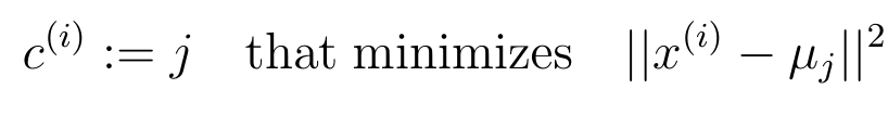
K-means算法流程：

找到最近的簇中心：

编写簇中心寻找程序findClosestCentroids.py：

import numpy as np


def find_closest_centroids(X, centroids):
    # Set K
    K = centroids.shape[0]#聚类中心数量

    m = X.shape[0]#样本数

    # You need to return the following variables correctly.
    idx = np.zeros(m)

    # ===================== Your Code Here =====================
    # Instructions : Go over every example, find its closest centroid, and store
    #                the index inside idx at the appropriate location.
    #                Concretely, idx[i] should contain the index of the centroid
    #                closest to example i. Hence, it should be a value in the
    #                range 0..k
    #
    distance = np.zeros((m,K))
    for i in range(m):#遍历样本
        for j in range(K):#遍历簇中心
            center = centroids[j]
            d = (X[i] - center) * (X[i] - center)
            distance[i, j] = d.sum()
    
    idx = np.argmin(distance, axis = 1)#返回聚类中心最近的中心的id

    # ==========================================================

    return idx

测试代码：

# ===================== Part 1: Find Closest Centroids =====================
# To help you implement K-means, we have divided the learning algorithm
# into two functions -- find_closest_centroids and compute_centroids. In this
# part, you should complete the code in the findClosestCentroids.py
#

print('Finding closest centroids.')

# Load an example dataset that we will be using
data = scio.loadmat('ex7data2.mat')
X = data['X']

# Select an initial set of centroids
k = 3  # Three centroids
initial_centroids = np.array([[3, 3], [6, 2], [8, 5]])

# Find the closest centroids for the examples using the
# initial_centroids
idx = fc.find_closest_centroids(X, initial_centroids)

print('Closest centroids for the first 3 examples: ')
print('{}'.format(idx[0:3]))
print('(the closest centroids should be 0, 2, 1 respectively)')

input('Program paused. Press ENTER to continue')

测试结果：

Finding closest centroids.
Closest centroids for the first 3 examples:
[0 2 1]
(the closest centroids should be 0, 2, 1 respectively)

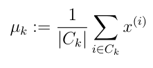
2.2计算均值

计算（更新）簇类中心（均值）：

编写代码computeCentroids.py：

import numpy as np


def compute_centroids(X, idx, K):
    # Useful values
    (m, n) = X.shape

    # You need to return the following variable correctly.
    centroids = np.zeros((K, n))

    # ===================== Your Code Here =====================
    # Instructions: Go over every centroid and compute mean of all points that
    #               belong to it. Concretely, the row vector centroids[i]
    #               should contain the mean of the data points assigned to
    #               centroid i.
    #
    for k in range(K):
        cluster = X[np.where(idx == k)]#找到每一类的样本
        cluster_sum = cluster.sum(axis = 0)/cluster.shape[0]#按列求和除该类样本总数
        centroids[k,:] = cluster_sum
    # ==========================================================

    return centroids

测试代码：

# ===================== Part 2: Compute Means =====================
# After implementing the closest centroids function, you should now
# complete the compute_centroids function.
#

print('Computing centroids means.')

# Compute means based on the closest centroids found in the previous part.
centroids = cc.compute_centroids(X, idx, k)

print('Centroids computed after initial finding of closest centroids: \n{}'.format(centroids))
print('the centroids should be')
print('[[ 2.428301 3.157924 ]')
print(' [ 5.813503 2.633656 ]')
print(' [ 7.119387 3.616684 ]]')

input('Program paused. Press ENTER to continue')

测试结果：

Computing centroids means.
Centroids computed after initial finding of closest centroids:
[[ 2.428301 3.157924]
[ 5.813503 2.633656]
[ 7.119387 3.616684]]
the centroids should be
[[ 2.428301 3.157924 ]
[ 5.813503 2.633656 ]
[ 7.119387 3.616684 ]]

2.3运行K-means聚类

查看runKMeans.py：

import numpy as np
import matplotlib.pyplot as plt
import matplotlib.colors as colors
import matplotlib.cm as cmx
import findClosestCentroids as fc
import computeCentroids as cc


def run_kmeans(X, initial_centroids, max_iters, plot):
    if plot:
        plt.figure()

    # Initialize values
    (m, n) = X.shape
    K = initial_centroids.shape[0]
    centroids = initial_centroids
    previous_centroids = centroids
    idx = np.zeros(m)

    # Run K-Means
    for i in range(max_iters):
        # Output progress
        print('K-Means iteration {}/{}'.format((i + 1), max_iters))

        # For each example in X, assign it to the closest centroid
        idx = fc.find_closest_centroids(X, centroids)#第一个内循环 为每个样本找到最近的聚类中心

        # Optionally plot progress
        if plot:
            plot_progress(X, centroids, previous_centroids, idx, K, i)
            previous_centroids = centroids
            input('Press ENTER to continue')

        # Given the memberships, compute new centroids
        centroids = cc.compute_centroids(X, idx, K)

    return centroids, idx#返回最终聚类中心的位置  和每个样本所属的聚类中心序号


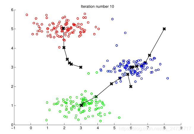
def plot_progress(X, centroids, previous, idx, K, i):
    plt.scatter(X[:, 0], X[:, 1], c=idx, s=15) #不同聚类中心用不同的颜色表示 

    plt.scatter(centroids[:, 0], centroids[:, 1], marker='x', c='black', s=25)#标出聚类中心

    for j in range(centroids.shape[0]): #为更新后的聚类中心和之前的聚类中心连线
        draw_line(centroids[j], previous[j])

    plt.title('Iteration number {}'.format(i + 1))


def draw_line(p1, p2):
    plt.plot(np.array([p1[0], p2[0]]), np.array([p1[1], p2[1]]), c='black', linewidth=1)

测试代码：

# ===================== Part 3: K-Means Clustering =====================
# After you have completed the two functions compute_centroids and
# find_closest_centroids, you will have all the necessary pieces to run the
# kMeans algorithm. In this part, you will run the K-Means algorithm on
# the example dataset we have provided.
#
print('Running K-Means Clustering on example dataset.')

# Load an example dataset
data = scio.loadmat('ex7data2.mat')
X = data['X']

# Settings for running K-Means
K = 3
max_iters = 10

# For consistency, here we set centroids to specific values
# but in practice you want to generate them automatically, such as by
# settings them to be random examples (as can be seen in
# kMeansInitCentroids).
initial_centroids = np.array([[3, 3], [6, 2], [8, 5]])

# Run K-Means algorithm. The 'true' at the end tells our function to plot
# the progress of K-Means
centroids, idx = km.run_kmeans(X, initial_centroids, max_iters, True)
print('K-Means Done.')

input('Program paused. Press ENTER to continue')

测试结果：

2.4随机初始化

编写随机初始化kMeansInitCentroids.py：

import numpy as np


def kmeans_init_centroids(X, K):
    # You should return this value correctly
    centroids = np.zeros((K, X.shape[1]))

    # ===================== Your Code Here =====================
    # Instructions: You should set centroids to randomly chosen examples from
    #               the dataset X
    #
    indices = np.random.randint(X.shape[0], size=K)

    #初始化聚类中心为数据集中的样本点
    centroids = X[indices]
    # ==========================================================

    return centroids

测试代码：

# ===================== Part 4: K-Means Clustering on Pixels =====================
#  In this exercise, you will use K-Means to compress an image. To do this,
#  you will first run K-Means on the colors of the pixels in the image and
#  then you will map each pixel onto its closest centroid.
#
#  You should now complete the code in kMeansInitCentroids.m
#
print('Running K-Means clustering on pixels from an image')

# Load an image of a bird
image = io.imread('bird_small.png')
image = img_as_float(image)

# Size of the image
img_shape = image.shape

# Reshape the image into an Nx3 matrix where N = number of pixels.
# Each row will contain the Red, Green and Blue pixel values
# This gives us our dataset matrix X that we will use K-Means on.

X = image.reshape(img_shape[0] * img_shape[1], 3)

# Run your K-Means algorithm on this data
# You should try different values of K and max_iters here
K = 16
max_iters = 10

# When using K-Means, it is important the initialize the centroids
# randomly.
# You should complete the code in kMeansInitCentroids.py before proceeding
initial_centroids = kmic.kmeans_init_centroids(X, K)

# Run K-Means
centroids, idx = km.run_kmeans(X, initial_centroids, max_iters, False)
print('K-Means Done.')

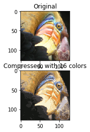
input('Program paused. Press ENTER to continue')

2.5图像压缩

测试代码：

# ===================== Part 5: Image Compression =====================
# In this part of the exercise, you will use the clusters of K-Means to
# compress an image. To do this, we first find the closest clusters for
# each example.
print('Applying K-Means to compress an image.')

# Find closest cluster members
idx = fc.find_closest_centroids(X, centroids)

# Essentially, now we have represented the image X as in terms of the
# indices in idx.

# We can now recover the image from the indices (idx) by mapping each pixel
# (specified by its index in idx) to the centroid value
X_recovered = centroids[idx]

# Reshape the recovered image into proper dimensions
X_recovered = np.reshape(X_recovered, (img_shape[0], img_shape[1], 3))

plt.subplot(2, 1, 1)
plt.imshow(image)
plt.title('Original')

plt.subplot(2, 1, 2)
plt.imshow(X_recovered)
plt.title('Compressed, with {} colors'.format(K))

input('ex7 Finished. Press ENTER to exit')

测试结果：

3.主成分分析

导入需要的包以及初始化：

import matplotlib.pyplot as plt
import numpy as np
import scipy.io as scio
from mpl_toolkits.mplot3d import Axes3D
from skimage import io
from skimage import img_as_float
import featureNormalize as fn
import pca as pca
import runkMeans as rk
import projectData as pd
import recoverData as rd
import displayData as disp
import kMeansInitCentroids as kmic
import runkMeans as km

plt.ion()
np.set_printoptions(formatter={'float': '{: 0.6f}'.format})

加载数据并可视化：

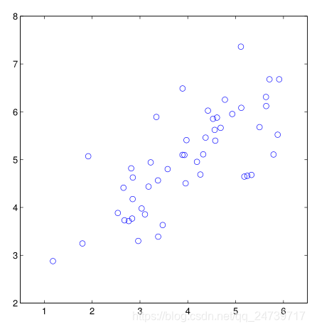
# ===================== Part 1: Load Example Dataset =====================
# We start this exercise by using a small dataset that is easily to
# visualize
#
print('Visualizing example dataset for PCA.')

# The following command loads the dataset.
data = scio.loadmat('ex7data1.mat')
X = data['X']

# Visualize the example dataset
plt.figure()
plt.scatter(X[:, 0], X[:, 1], facecolors='none', edgecolors='b', s=20)
plt.axis('equal')
plt.axis([0.5, 6.5, 2, 8])

input('Program paused. Press ENTER to continue')

测试结果：

3.1实现PCA

查看特征缩放程序featureNormalize.py：

def feature_normalize(X):
    mu = np.mean(X, 0)  #对特征矩阵每一列求均值
    sigma = np.std(X, 0, ddof=1)  #特征矩阵每一列求标准差
    X_norm = (X - mu) / sigma  #特征矩阵每一列的元素减去该列均值  除以该列标准差  得到特征缩放后的矩阵
 
    return X_norm, mu, sigma

编写pca.py：

import numpy as np
import scipy


def pca(X):
    # Useful values
    (m, n) = X.shape

    # You need to return the following variables correctly.
    U = np.zeros(n)
    S = np.zeros(n)

    # ===================== Your Code Here =====================
    # Instructions: You should first compute the covariance matrix. Then, you
    #               should use the 'scipy.linalg.svd' function to compute the eigenvectors
    #               and eigenvalues of the covariance matrix.
    #
    # Note: When computing the covariance matrix, remember to divide by m (the
    #       number of examples).
    # 
    # Hint: Take a look at full_matrices, compute_uv parameters for the svd function
    #
    covariance = (1/m)*np.dot(X.T, X)

    #对协方差矩阵进行奇异值分解
    U,S,_ = scipy.linalg.svd(covariance)

    # ==========================================================

    return U, S

测试代码：

# ===================== Part 2: Principal Component Analysis =====================
# You should now implement PCA, a dimension reduction technique. You
# should complete the code in pca.py
#
print('Running PCA on example dataset.')

# Before running PCA, it is important to first normalize X
X_norm, mu, sigma = fn.feature_normalize(X)

# Run PCA
U, S = pca.pca(X_norm)

rk.draw_line(mu, mu + 1.5 * S[0] * U[:, 0])
rk.draw_line(mu, mu + 1.5 * S[1] * U[:, 1])

print('Top eigenvector: \nU[:, 0] = {}'.format(U[:, 0]))
print('You should expect to see [-0.707107 -0.707107]')

input('Program paused. Press ENTER to continue')

可视化降维后的特征向量（子空间的基向量）及测试结果：

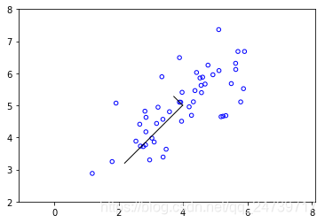
Running PCA on example dataset.
Top eigenvector:
U[:, 0] = [-0.707107 -0.707107]
You should expect to see [-0.707107 -0.707107]

3.2PCA降维

编写降维程序projectData.py：

import numpy as np


def project_data(X, U, K):
    # You need to return the following variables correctly.
    Z = np.zeros((X.shape[0], K))#降维后的特征矩阵 Z：m*K X：m*n

    # ===================== Your Code Here =====================
    # Instructions: Compute the projection of the data using only the top K
    #               eigenvectors in U (first K columns).
    #               For the i-th example X[i], the projection on to the k-th
    #               eigenvector is given as follows:
    #                   x = X(i, :)';
    #                   projection_k = x' * U(:, k);
    #                   (above is octave code)
    #
    Ureduce = U[:, np.arange(K)]
    Z = np.dot(X, Ureduce)


    # ==========================================================

    return Z

编写压缩重放程序recoverData.py：

import numpy as np


def recover_data(Z, U, K):
    # You need to return the following variables correctly.
    X_rec = np.zeros((Z.shape[0], U.shape[0]))#原始样本在特征向量上的投影点 X_rec:m*n Z:m*K  U:n*n

    # ===================== Your Code Here =====================
    # Instructions: Compute the approximation of the data by projecting back
    #               onto the original space using the top K eigenvectors in U.
    #
    #               For the i-th example Z[i], the approximate
    #               recovered data for dimension j is given as follows:
    #                   v = Z(i, :)';
    #                   recovered_j = v' * U(j, 1:K)';
    #                   (above is octave code)
    #
    Ureduce = U[:, np.arange(K)]
    X_rec = np.dot(Z, Ureduce.T)

    # ==========================================================

    return X_rec

测试代码：

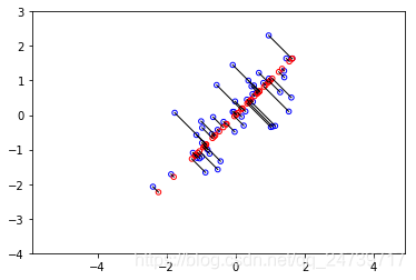
# ===================== Part 3: Dimension Reduction =====================
# You should now implement the projection step to map the data onto the
# first k eigenvectors. The code will then plot the data in this reduced
# dimensional space. This will show you what the data looks like when
# using only the correspoding eigenvectors to reconstruct it.
#
# You should complete the code in projectData.py
#
print('Dimension reductino on example dataset.')

# Plot the normalized dataset (returned from pca)
plt.figure()
plt.scatter(X_norm[:, 0], X_norm[:, 1], facecolors='none', edgecolors='b', s=20)
plt.axis('equal')
plt.axis([-4, 3, -4, 3])

# Project the data onto K = 1 dimension
K = 1
Z = pd.project_data(X_norm, U, K)
print('Projection of the first example: {}'.format(Z[0]))
print('(this value should be about 1.481274)')

X_rec = rd.recover_data(Z, U, K)

print('Approximation of the first example: {}'.format(X_rec[0]))
print('(this value should be about [-1.047419 -1.047419])')

# Draw lines connecting the projected points to the original points
plt.scatter(X_rec[:, 0], X_rec[:, 1], facecolors='none', edgecolors='r', s=20)
for i in range(X_norm.shape[0]):
    rk.draw_line(X_norm[i], X_rec[i])
 
input('Program paused. Press ENTER to continue')

测试结果：

Dimension reductino on example dataset.
Projection of the first example: [ 1.481274]
(this value should be about 1.481274)
Approximation of the first example: [-1.047419 -1.047419]
(this value should be about [-1.047419 -1.047419])

3.3脸图像数据集

加载数据：

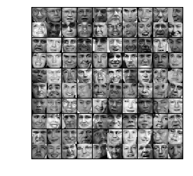
# ===================== Part 4: Loading and Visualizing Face Data =====================
# We start the exercise by first loading and visualizing the dataset.
# The following code will load the dataset into your environment
#
print('Loading face dataset.')

# Load Face dataset
data = scio.loadmat('ex7faces.mat')
X = data['X']

disp.display_data(X[0:100])

input('Program paused. Press ENTER to continue')

可视化结果：

可视化人脸数据的特征向量：

# ===================== Part 5: PCA on Face Data: Eigenfaces =====================
# Run PCA and visualize the eigenvectors which are in this case eigenfaces
# We display the first 36 eigenfaces.
#
print('Running PCA on face dataset.\n(this might take a minute or two ...)')

# Before running PCA, it is important to first normalize X by subtracting
# the mean value from each feature
X_norm, mu, sigma = fn.feature_normalize(X)

# Run PCA
U, S = pca.pca(X_norm)

# Visualize the top 36 eigenvectors found
disp.display_data(U[:, 0:36].T)

input('Program paused. Press ENTER to continue')

可视化效果：

人脸数据降维（1024-->100）：

# ===================== Part 6: Dimension Reduction for Faces =====================
# Project images to the eigen space using the top k eigenvectors
# If you are applying a machine learning algorithm
print('Dimension reduction for face dataset.')

K = 100
Z = pd.project_data(X_norm, U, K)

print('The projected data Z has a shape of: {}'.format(Z.shape))

input('Program paused. Press ENTER to continue')

可视化降维后，再压缩重放后的人脸数据与原数据比较：


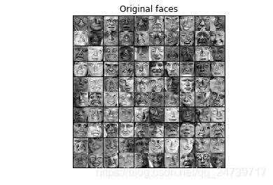
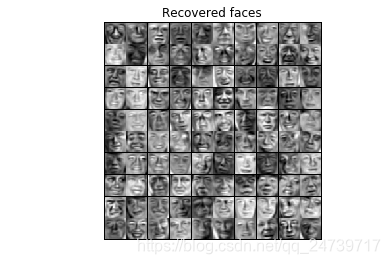
# =========== Part 7: Visualization of Faces after PCA Dimension Reduction ===========
# Project images to the eigen space using the top K eigen vectors and
# visualize only using those K dimensions
# Compare to the original input, which is also displayed
print('Visualizing the projected (reduced dimension) faces.')

K = 100
X_rec = rd.recover_data(Z, U, K)

# Display normalized data
disp.display_data(X_norm[0:100])
plt.title('Original faces')
plt.axis('equal')

# Display reconstructed data from only k eigenfaces
disp.display_data(X_rec[0:100])
plt.title('Recovered faces')
plt.axis('equal')

input('Program paused. Press ENTER to continue')

测试结果：

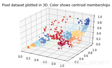
利用PCA可视化高维数据:

# ===================== Part 8(a): PCA for Visualization =====================
# One useful application of PCA is to use it to visualize high-dimensional
# data. In the last K-Means exercise you ran K-Means on 3-dimensional
# pixel colors of an image. We first visualize this output in 3D, and then
# apply PCA to obtain a visualization in 2D.

# Reload the image from the previous exercise and run K-Means on it
# For this to work, you need to complete the K-Means assignment first
image = io.imread('bird_small.png')
image = img_as_float(image)

img_shape = image.shape

X = image.reshape((img_shape[0] * img_shape[1], 3)) #将图片格式转换为包含3列（3个颜色通道）的矩阵
K = 16 #聚类中心数量
max_iters = 10
initial_centroids = kmic.kmeans_init_centroids(X, K) #初始化K个聚类中心
centroids, idx = km.run_kmeans(X, initial_centroids, max_iters, False)#执行k-means，得到最终的聚类中心和每个样本点所属的聚类中心序号

# Sample 1000 random indices (since working with all the data is
# too expensive. If you have a fast computer, you may increase this.
selected = np.random.randint(X.shape[0], size=1000)

# Visualize the data and centroid memberships in 3D
cm = plt.cm.get_cmap('RdYlBu')
fig = plt.figure()
ax = fig.add_subplot(111, projection='3d')
ax.scatter(X[selected, 0], X[selected, 1], X[selected, 2], c=idx[selected].astype(np.float64), s=15, cmap=cm, vmin=0, vmax=K)
plt.title('Pixel dataset plotted in 3D. Color shows centroid memberships')

input('Program paused. Press ENTER to continue')

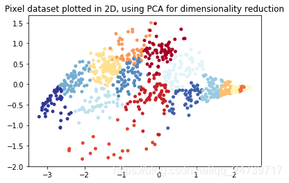
# ===================== Part 8(b): PCA for Visualization =====================
# Use PCA to project this cloud to 2D for visualization

#利用PCA把3维数据 降至2维 进行可视化
X_norm, mu, sigma = fn.feature_normalize(X)

# PCA and project the data to 2D
U, S = pca.pca(X_norm)
Z = pd.project_data(X_norm, U, 2)#得到降维后的特征矩阵

# Plot in 2D
plt.figure()
plt.scatter(Z[selected, 0], Z[selected, 1], c=idx[selected].astype(np.float64), s=15, cmap=cm)
plt.title('Pixel dataset plotted in 2D, using PCA for dimensionality reduction')

input('ex7_pca Finished. Press ENTER to exit')

测试结果：

NotFound1911

关注

1
点赞
踩
1

收藏

觉得还不错? 一键收藏
0
评论
吴恩达cs229|编程作业第七周（Python）

练习七：k均值聚类与主成分分析目录：1.包含的文件。2.k均值聚类。3.（PCA）主成成分分析。1.包含的文件。文件名含义 ex7.py K-means实验 ex7_pca.py PCA实验 ex7data1.mat PCA实验数据集 ex7data2.mat K-means实验数据集 ex7faces...
复制链接

扫一扫