Batch Normalization论文详解

翻译论文汇总

Batch Normalization: Accelerating Deep Network Training by Reducing Internal Covariate Shift

Abstract

Training Deep Neural Networks is complicated by the fact that the distribution of each layer’s inputs changes during training, as the parameters of the previous layers change. This slows down the training by requiring lower learning rates and careful parameter initialization, and makes it notoriously hard to train models with saturating nonlinearities. We refer to this phenomenon as internal covariate shift, and address the problem by normalizing layer inputs. Our method draws its strength from making normalization a part of the model architecture and performing the normalization for each training mini-batch. Batch Normalization allows us to use much higher learning rates and be less careful about initialization. It also acts as a regularizer, in some cases eliminating the need for Dropout. Applied to a state-of-the-art image classification model, Batch Normalization achieves the same accuracy with 14 times fewer training steps, and beats the original model by a significant margin. Using an ensemble of batch-normalized networks, we improve upon the best published result on ImageNet classification: reaching 4.9% top-5 validation error (and 4.8% test error), exceeding the accuracy of human raters.

摘要

训练深度神经网络的复杂性在于，每层输入的分布在训练过程中会发生变化，因为前面的层的参数会发生变化。通过要求较低的学习率和仔细的参数初始化减慢了训练，并且使具有饱和非线性的模型训练起来非常困难。我们将这种现象称为内部协变量转移，并通过标准化层输入来解决这个问题。我们的方法力图使标准化成为模型架构的一部分，并为每个训练小批量数据执行标准化。批标准化使我们能够使用更高的学习率，并且不用太注意初始化。它也作为一个正则化项，在某些情况下不需要Dropout。将批量标准化应用到最先进的图像分类模型上，批标准化在取得相同的精度的情况下，减少了14倍的训练步骤，并以显著的差距击败了原始模型。使用批标准化网络的组合，我们改进了在ImageNet分类上公布的最佳结果：达到了4.9％ top-5的验证误差（和4.8％测试误差），超过了人类评估者的准确性。

1. Introduction

Deep learning has dramatically advanced the state of the art in vision, speech, and many other areas. Stochastic gradient descent (SGD) has proved to be an effective way of training deep networks, and SGD variants such as momentum (Sutskever et al., 2013) and Adagrad (Duchi et al., 2011) have been used to achieve state of the art performance. SGD optimizes the parameters $\Theta$ of the network, so as to minimize the loss

$$\Theta =\arg \underset{\Theta }{\min }\frac{1}{N}\sum _{i=1}^N\ell (x_i,\Theta )$$

where $x_{1\dots N}$ is the training data set. With SGD, the training proceeds in steps, and at each step we consider a mini-batch $x_{1\dots m}$ of size $m$. The mini-batch is used to approximate the gradient of the loss function with respect to the parameters, by computing $\frac{1}{m}{\sum }_{i=1}^m\frac{\partial \ell (x_i,\Theta )}{\partial \Theta }$. Using mini-batches of examples, as opposed to one example at a time, is helpful in several ways. First, the gradient of the loss over a mini-batch is an estimate of the gradient over the training set, whose quality improves as the batch size increases. Second, computation over a batch can be much more efficient than $m$ computations for individual examples, due to the parallelism afforded by the modern computing platforms.

1. 引言

深度学习在视觉、语音等诸多方面显著提高了现有技术的水平。随机梯度下降（SGD）已经被证明是训练深度网络的有效方式，并且已经使用诸如动量（Sutskever等，2013）和Adagrad（Duchi等人，2011）等SGD变种取得了最先进的性能。SGD优化网络参数$\Theta$，以最小化损失

$$\Theta =\arg \underset{\Theta }{\min }\frac{1}{N}\sum _{i=1}^N\ell (x_i,\Theta )$$

$x_{1\dots N}$是训练数据集。使用SGD，训练将逐步进行，在每一步中，我们考虑一个大小为$m$的小批量数据$x_{1\dots m}$。通过计算$\frac{1}{m}{\sum }_{i=1}^m\frac{\partial \ell (x_i,\Theta )}{\partial \Theta }$，使用小批量数据来近似损失函数关于参数的梯度。使用小批量样本，而不是一次一个样本，在一些方面是有帮助的。首先，小批量数据的梯度损失是训练集上的梯度估计，其质量随着批量增加而改善。第二，由于现代计算平台提供的并行性，对一个批次的计算比单个样本计算$m$次效率更高。

While stochastic gradient is simple and effective, it requires careful tuning of the model hyper-parameters, specifically the learning rate used in optimization, as well as the initial values for the model parameters. The training is complicated by the fact that the inputs to each layer are affected by the parameters of all preceding layers —— so that small changes to the network parameters amplify as the network becomes deeper.

虽然随机梯度是简单有效的，但它需要仔细调整模型的超参数，特别是优化中使用的学习速率以及模型参数的初始值。训练的复杂性在于每层的输入受到前面所有层的参数的影响——因此当网络变得更深时，网络参数的微小变化就会被放大。

The change in the distributions of layers’ inputs presents a problem because the layers need to continuously adapt to the new distribution. When the input distribution to a learning system changes, it is said to experience covariate shift (Shimodaira, 2000). This is typically handled via domain adaptation (Jiang, 2008). However, the notion of covariate shift can be extended beyond the learning system as a whole, to apply to its parts, such as a sub-network or a layer. Consider a network computing $$\ell =F_2(F_1(u,{\Theta }_1),{\Theta }_2)$$ where $F_1$ and $F_2$ are arbitrary transformations, and the parameters ${\Theta }_1,{\Theta }_2$ are to be learned so as to minimize the loss $\ell$. Learning ${\Theta }_2$ can be viewed as if the inputs $x=F_1(u,{\Theta }_1)$ are fed into the sub-network $$\ell =F_2(x,{\Theta }_2).$$

层输入的分布变化是一个问题，因为这些层需要不断适应新的分布。当学习系统的输入分布发生变化时，据说会经历协变量转移（Shimodaira，2000）。这通常是通过域适应（Jiang，2008）来处理的。然而，协变量漂移的概念可以扩展到整个学习系统之外，应用到学习系统的一部分，例如子网络或一层。考虑网络计算$$\ell =F_2(F_1(u,{\Theta }_1),{\Theta }_2)$$ $F_1$和$F_2$是任意变换，学习参数${\Theta }_1，{\Theta }_2$以便最小化损失$\ell$。学习${\Theta }_2$可以看作输入$x=F_1(u,{\Theta }_1)$送入到子网络$$\ell =F_2(x,{\Theta }_2)。$$

For example, a gradient descent step $${\Theta }_2\leftarrow {\Theta }_2-\frac{\alpha }{m}\sum _{i=1}^m\frac{\partial F_2(x_i,{\Theta }_2)}{\partial {\Theta }_2}$$ (for batch size $m$ and learning rate $\alpha$) is exactly equivalent to that for a stand-alone network $F_2$ with input $x$. Therefore, the input distribution properties that make training more efficient —— such as having the same distribution between the training and test data —— apply to training the sub-network as well. As such it is advantageous for the distribution of $x$ to remain fixed over time. Then, ${\Theta }_2$ does not have to readjust to compensate for the change in the distribution of $x$.

例如，梯度下降步骤$${\Theta }_2\leftarrow {\Theta }_2-\frac{\alpha }{m}\sum _{i=1}^m\frac{\partial F_2(x_i,{\Theta }_2)}{\partial {\Theta }_2}$$（对于批大小$m$和学习率$\alpha$）与输入为$x$的单独网络$F_2$完全等价。因此，输入分布特性使训练更有效——例如训练数据和测试数据之间有相同的分布——也适用于训练子网络。因此$x$的分布在时间上保持固定是有利的。然后，${\Theta }_2$不必重新调整来补偿$x$分布的变化。

Fixed distribution of inputs to a sub-network would have positive consequences for the layers outside the sub-network, as well. Consider a layer with a sigmoid activation function $z=g(Wu+b)$ where $u$ is the layer input, the weight matrix $W$ and bias vector $b$ are the layer parameters to be learned, and $g(x)=\frac{1}{1+\exp (-x)}$. As $|x|$ increases, $g^{\prime }(x)$ tends to zero. This means that for all dimensions of $x=Wu+b$ except those with small absolute values, the gradient flowing down to $u$ will vanish and the model will train slowly. However, since $x$ is affected by $W,b$ and the parameters of all the layers below, changes to those parameters during training will likely move many dimensions of $x$ into the saturated regime of the nonlinearity and slow down the convergence. This effect is amplified as the network depth increases. In practice, the saturation problem and the resulting vanishing gradients are usually addressed by using Rectified Linear Units (Nair & Hinton, 2010) $ReLU(x)=\max (x,0)$, careful initialization (Bengio & Glorot, 2010; Saxe et al., 2013), and small learning rates. If, however, we could ensure that the distribution of nonlinearity inputs remains more stable as the network trains, then the optimizer would be less likely to get stuck in the saturated regime, and the training would accelerate.

子网络输入的固定分布对于子网络外的层也有积极的影响。考虑一个激活函数为$g(x)=\frac{1}{1+\exp (-x)}$的层，$u$是层输入，权重矩阵$W$和偏置向量$b$是要学习的层参数，$g(x)=\frac{1}{1+\exp (-x)}$。随着$|x|$的增加，$g^{\prime }(x)$趋向于0。这意味着对于$x=Wu+b$的所有维度，除了那些具有小的绝对值之外，流向$u$的梯度将会消失，模型将缓慢的进行训练。然而，由于$x$受$W,b$和下面所有层的参数的影响，训练期间那些参数的改变可能会将$x$的许多维度移动到非线性的饱和状态并减慢收敛。这个影响随着网络深度的增加而放大。在实践中，饱和问题和由此产生的梯度消失通常通过使用修正线性单元(Nair & Hinton, 2010) $ReLU(x)=\max (x,0)$，仔细的初始化(Bengio & Glorot, 2010; Saxe et al., 2013)和小的学习率来解决。然而，如果我们能保证非线性输入的分布在网络训练时保持更稳定，那么优化器将不太可能陷入饱和状态，训练将加速。

We refer to the change in the distributions of internal nodes of a deep network, in the course of training, as Internal Covariate Shift. Eliminating it offers a promise of faster training. We propose a new mechanism, which we call Batch Normalization, that takes a step towards reducing internal covariate shift, and in doing so dramatically accelerates the training of deep neural nets. It accomplishes this via a normalization step that fixes the means and variances of layer inputs. Batch Normalization also has a beneficial effect on the gradient flow through the network, by reducing the dependence of gradients on the scale of the parameters or of their initial values. This allows us to use much higher learning rates without the risk of divergence. Furthermore, batch normalization regularizes the model and reduces the need for Dropout (Srivastava et al., 2014). Finally, Batch Normalization makes it possible to use saturating nonlinearities by preventing the network from getting stuck in the saturated modes.

我们把训练过程中深度网络内部结点的分布变化称为内部协变量转移。消除它可以保证更快的训练。我们提出了一种新的机制，我们称为为批标准化，它是减少内部协变量转移的一个步骤，这样做可以显著加速深度神经网络的训练。它通过标准化步骤来实现，标准化步骤修正了层输入的均值和方差。批标准化减少了梯度对参数或它们的初始值尺度上的依赖，对通过网络的梯度流动有有益的影响。这允许我们使用更高的学习率而没有发散的风险。此外，批标准化使模型正则化并减少了对Dropout(Srivastava et al., 2014)的需求。最后，批标准化通过阻止网络陷入饱和模式让使用饱和非线性成为可能。

In Sec. 4.2, we apply Batch Normalization to the best-performing ImageNet classification network, and show that we can match its performance using only 7% of the training steps, and can further exceed its accuracy by a substantial margin. Using an ensemble of such networks trained with Batch Normalization, we achieve the top-5 error rate that improves upon the best known results on ImageNet classification.

在4.2小节，我们将批标准化应用到性能最好的ImageNet分类网络上，并且表明我们可以使用仅7％的训练步骤来匹配其性能，并且可以进一步超过其准确性一大截。通过使用批标准化训练的网络的集合，我们取得了top-5错误率，其改进了ImageNet分类上已知的最佳结果。

2. Towards Reducing Internal Covariate Shift

We define Internal Covariate Shift as the change in the distribution of network activations due to the change in network parameters during training. To improve the training, we seek to reduce the internal covariate shift. By fixing the distribution of the layer inputs $x$ as the training progresses, we expect to improve the training speed. It has been long known (LeCun et al., 1998b; Wiesler & Ney, 2011) that the network training converges faster if its inputs are whitened – i.e., linearly transformed to have zero means and unit variances, and decorrelated. As each layer observes the inputs produced by the layers below, it would be advantageous to achieve the same whitening of the inputs of each layer. By whitening the inputs to each layer, we would take a step towards achieving the fixed distributions of inputs that would remove the ill effects of the internal covariate shift.

2. 减少内部协变量转变

由于训练过程中网络参数的变化，我们将内部协变量转移定义为网络激活分布的变化。为了改善训练，我们寻求减少内部协变量转移。随着训练的进行，通过固定层输入$x$的分布，我们期望提高训练速度。众所周知(LeCun et al., 1998b; Wiesler & Ney, 2011)如果对网络的输入进行白化，网络训练将会收敛的更快——即输入线性变换为具有零均值和单位方差，并去相关。当每一层观察下面的层产生的输入时，实现每一层输入进行相同的白化将是有利的。通过白化每一层的输入，我们将采取措施实现输入的固定分布，消除内部协变量转移的不良影响。

We could consider whitening activations at every training step or at some interval, either by modifying the network directly or by changing the parameters of the optimization algorithm to depend on the network activation values (Wiesler et al., 2014; Raiko et al., 2012; Povey et al., 2014; Desjardins & Kavukcuoglu). However, if these modifications are interspersed with the optimization steps, then the gradient descent step may attempt to update the parameters in a way that requires the normalization to be updated, which reduces the effect of the gradient step. For example, consider a layer with the input $u$ that adds the learned bias $b$, and normalizes the result by subtracting the mean of the activation computed over the training data: $\hat{x}=x-E[x]$ where $x=u+b$, $X=x_{1\dots N}$ is the set of values of $x$ over the training set, and $E[x]=\frac{1}{N}{\sum }_{i=1}^N{x}_i$. If a gradient descent step ignores the dependence of $E[x]$ on $b$, then it will update $b\leftarrow b+\Delta b$, where $\Delta b\propto -\partial \ell /\partial \hat{x}$. Then $u+(b+\Delta b)-E[u+(b+\Delta b)]=u+b-E[u+b]$. Thus, the combination of the update to $b$ and subsequent change in normalization led to no change in the output of the layer nor, consequently, the loss. As the training continues, $b$ will grow indefinitely while the loss remains fixed. This problem can get worse if the normalization not only centers but also scales the activations. We have observed this empirically in initial experiments, where the model blows up when the normalization parameters are computed outside the gradient descent step.

我们考虑在每个训练步骤或在某些间隔来白化激活值，通过直接修改网络或根据网络激活值来更改优化方法的参数(Wiesler et al., 2014; Raiko et al., 2012; Povey et al., 2014; Desjardins & Kavukcuoglu)。然而，如果这些修改分散在优化步骤中，那么梯度下降步骤可能会试图以要求标准化进行更新的方式来更新参数，这会降低梯度下降步骤的影响。例如，考虑一个层，其输入$u$加上学习到的偏置$b$，通过减去在训练集上计算的激活值的均值对结果进行归一化：$\hat{x}=x-E[x]$，$x=u+b$, $X=x_{1\dots N}$是训练集上$x$值的集合，$E[x]=\frac{1}{N}{\sum }_{i=1}^N{x}_i$。如果梯度下降步骤忽略了$E[x]$对$b$的依赖，那它将更新$b\leftarrow b+\Delta b$，其中$\Delta b\propto -\partial \ell /\partial \hat{x}$。然后$u+(b+\Delta b)-E[u+(b+\Delta b)]=u+b-E[u+b]$。因此，结合$b$的更新和接下来标准化中的改变会导致层的输出没有变化，从而导致损失没有变化。随着训练的继续，$b$将无限增长而损失保持不变。如果标准化不仅中心化而且缩放了激活值，问题会变得更糟糕。我们在最初的实验中已经观察到了这一点，当标准化参数在梯度下降步骤之外计算时，模型会爆炸。

The issue with the above approach is that the gradient descent optimization does not take into account the fact that the normalization takes place. To address this issue, we would like to ensure that, for any parameter values, the network always produces activations with the desired distribution. Doing so would allow the gradient of the loss with respect to the model parameters to account for the normalization, and for its dependence on the model parameters $\Theta$. Let again $x$ be a layer input, treated as a vector, and $X$ be the set of these inputs over the training data set. The normalization can then be written as a transformation $$\hat{x}=Norm(x,X)$$ which depends not only on the given training example $x$ but on all examples $X$ – each of which depends on $\Theta$ if $x$ is generated by another layer. For backpropagation, we would need to compute the Jacobians $\frac{\partial Norm(x,X)}{\partial x}$ and $\frac{\partial Norm(x,X)}{\partial X}$; ignoring the latter term would lead to the explosion described above. Within this framework, whitening the layer inputs is expensive, as it requires computing the covariance matrix $Cov[x]=E_{x\in X}[x{x}^T]-E[x]E[x{]}^T$ and its inverse square root, to produce the whitened activations $Cov[x{]}^{-1/2}(x-E[x])$, as well as the derivatives of these transforms for backpropagation. This motivates us to seek an alternative that performs input normalization in a way that is differentiable and does not require the analysis of the entire training set after every parameter update.

上述方法的问题是梯度下降优化没有考虑到标准化中发生的事实。为了解决这个问题，我们希望确保对于任何参数值，网络总是产生具有所需分布的激活值。这样做将允许关于模型参数损失的梯度来解释标准化，以及它对模型参数$\Theta$的依赖。设$x$为层的输入，将其看作向量，$X$是这些输入在训练集上的集合。标准化可以写为变换$$\hat{x}=Norm(x,X)$$它不仅依赖于给定的训练样本$x$而且依赖于所有样本$X$——它们中的每一个都依赖于$\Theta$，如果$x$是由另一层生成的。对于反向传播，我们将需要计算雅可比行列式$\frac{\partial Norm(x,X)}{\partial x}$和$\frac{\partial Norm(x,X)}{\partial X}$；忽略后一项会导致上面描述的爆炸。在这个框架中，白化层输入是昂贵的，因为它要求计算协方差矩阵$Cov[x]=E_{x\in X}[x{x}^T]-E[x]E[x]T$和它的平方根倒数，从而生成白化的激活$Cov[x]-1/2(x-E[x])$和这些变换进行反向传播的偏导数。这促使我们寻求一种替代方案，以可微分的方式执行输入标准化，并且在每次参数更新后不需要对整个训练集进行分析。

Some of the previous approaches (e.g. (Lyu & Simoncelli, 2008)) use statistics computed over a single training example, or, in the case of image networks, over different feature maps at a given location. However, this changes the representation ability of a network by discarding the absolute scale of activations. We want to a preserve the information in the network, by normalizing the activations in a training example relative to the statistics of the entire training data.

以前的一些方法（例如（Lyu＆Simoncelli，2008））使用通过单个训练样本计算的统计信息，或者在图像网络的情况下，使用给定位置处不同特征图上的统计。然而，通过丢弃激活值绝对尺度改变了网络的表示能力。我们希望通过对相对于整个训练数据统计信息的单个训练样本的激活值进行归一化来保留网络中的信息。

3. Normalization via Mini-Batch Statistics

Since the full whitening of each layer’s inputs is costly and not everywhere differentiable, we make two necessary simplifications. The first is that instead of whitening the features in layer inputs and outputs jointly, we will normalize each scalar feature independently, by making it have the mean of zero and unit variance. For a layer with $d$-dimensional input $x=(x^{(1)}\dots x^{(d)})$, we will normalize each dimension $${\hat{x}}^{(k)}=\frac{x^{(k)}-E[x^{(k)}]}{\sqrt{Var[x^{(k)}]}}$$ where the expectation and variance are computed over the training data set. As shown in (LeCun et al., 1998b), such normalization speeds up convergence, even when the features are not decorrelated.

3. 通过Mini-Batch统计进行标准化

由于每一层输入的整个白化是代价昂贵的并且不是到处可微分的，因此我们做了两个必要的简化。首先是我们将单独标准化每个标量特征，从而代替在层输入输出对特征进行共同白化，使其具有零均值和单位方差。对于具有$d$维输入$x=(x^{(1)}\dots x^{(d)})$的层，我们将标准化每一维$${\hat{x}}^{(k)}=\frac{x^{(k)}-E[x^{(k)}]}{\sqrt{Var[x^{(k)}]}}$$其中期望和方差在整个训练数据集上计算。如(LeCun et al., 1998b)中所示，这种标准化加速了收敛，即使特征没有去相关。

Note that simply normalizing each input of a layer may change what the layer can represent. For instance, normalizing the inputs of a sigmoid would constrain them to the linear regime of the nonlinearity. To address this, we make sure that the transformation inserted in the network can represent the identity transform. To accomplish this, we introduce, for each activation $x^{(k)}$, a pair of parameters ${\gamma }^{(k)},{\beta }^{(k)}$, which scale and shift the normalized value: $$y^{(k)}={\gamma }^{(k)}{\hat{x}}^{(k)}+{\beta }^{(k)}.$$ These parameters are learned along with the original model parameters, and restore the representation power of the network. Indeed, by setting ${\gamma }^{(k)}=\sqrt{Var[x^{(k)}]}$ and ${\beta }^{(k)}=E[x^{(k)}]$, we could recover the original activations, if that were the optimal thing to do.

注意简单标准化层的每一个输入可能会改变层可以表示什么。例如，标准化sigmoid的输入会将它们约束到非线性的线性状态。为了解决这个问题，我们要确保插入到网络中的变换可以表示恒等变换。为了实现这个，对于每一个激活值$x(k)$，我们引入成对的参数$\gamma (k)，\beta (k)$，它们会归一化和移动标准化值：$$y(k)={\gamma }^{(k)}{\hat{x}}^{(k)}+\beta (k).$$这些参数与原始的模型参数一起学习，并恢复网络的表示能力。实际上，通过设置$\gamma (k)=\sqrt{Var[x(k)]}$和$\beta (k)=E[x^{(k)}]$，我们可以重新获得原始的激活值，如果这是要做的最优的事。

In the batch setting where each training step is based on the entire training set, we would use the whole set to normalize activations. However, this is impractical when using stochastic optimization. Therefore, we make the second simplification: since we use mini-batches in stochastic gradient training, each mini-batch produces estimates of the mean and variance of each activation. This way, the statistics used for normalization can fully participate in the gradient backpropagation. Note that the use of mini-batches is enabled by computation of per-dimension variances rather than joint covariances; in the joint case, regularization would be required since the mini-batch size is likely to be smaller than the number of activations being whitened, resulting in singular covariance matrices.

每个训练步骤的批处理设置是基于整个训练集的，我们将使用整个训练集来标准化激活值。然而，当使用随机优化时，这是不切实际的。因此，我们做了第二个简化：由于我们在随机梯度训练中使用小批量，每个小批量产生每次激活平均值和方差的估计。这样，用于标准化的统计信息可以完全参与梯度反向传播。注意，通过计算每一维的方差而不是联合协方差，可以实现小批量的使用；在联合情况下，将需要正则化，因为小批量大小可能小于白化的激活值的数量，从而导致单个协方差矩阵。

Consider a mini-batch $B$ of size $m$. Since the normalization is applied to each activation independently, let us focus on a particular activation $x^{(k)}$ and omit $k$ for clarity. We have $m$ values of this activation in the mini-batch, B = { x 1 … m } . \it B=\lbrace x_{1\ldots m} \rbrace. B={x1…m​}. Let the normalized values be ${\hat{x}}_{1\dots m}$, and their linear transformations be $y_{1\dots m}$. We refer to the transform $$B{N}_{\gamma ,\beta }:x_{1\dots m}\to y_{1\dots m}$$ as the Batch Normalizing Transform. We present the BN Transform in Algorithm 1. In the algorithm, $ϵ$ is a constant added to the mini-batch variance for numerical stability.

Algorithm 1
考虑一个大小为$m$的小批量数据$B$。由于标准化被单独地应用于每一个激活，所以让我们集中在一个特定的激活$x^{(k)}$，为了清晰，忽略$k$。在小批量数据里我们有这个激活的$m$个值， B = { x 1 … m } . \it B=\lbrace x_{1\ldots m} \rbrace. B={x1…m​}.设标准化值为${\hat{x}}_{1\dots m}$，它们的线性变换为$y_{1\dots m}$。我们把变换$$B{N}_{\gamma ,\beta }:x_{1\dots m}\to y_{1\dots m}$$看作批标准化变换。我们在算法1中提出了BN变换。在算法中，为了数值稳定，$ϵ$是一个加到小批量数据方差上的常量。

Algorithm 1
The BN transform can be added to a network to manipulate any activation. In the notation $y=B{N}_{\gamma ,\beta }(x)$, we indicate that the parameters $\gamma$ and $\beta$ are to be learned, but it should be noted that the BN transform does not independently process the activation in each training example. Rather, $B{N}_{\gamma ,\beta }(x)$ depends both on the training example and the other examples in the mini-batch. The scaled and shifted values $y$ are passed to other network layers. The normalized activations $\hat{x}$ are internal to our transformation, but their presence is crucial. The distributions of values of any $\hat{x}$ has the expected value of $0$ and the variance of $1$, as long as the elements of each mini-batch are sampled from the same distribution, and if we neglect $ϵ$. This can be seen by observing that ${\sum }_{i=1}^m{\hat{x}}_i=0$ and $\frac{1}{m}{\sum }_{i=1}^m{\hat{x}}_i^2=1$, and taking expectations. Each normalized activation ${\hat{x}}^{(k)}$ can be viewed as an input to a sub-network composed of the linear transform $y(k)=\gamma (k)\hat{x}(k)+\beta (k)$, followed by the other processing done by the original network. These sub-network inputs all have fixed means and variances, and although the joint distribution of these normalized ${\hat{x}}^{(k)}$ can change over the course of training, we expect that the introduction of normalized inputs accelerates the training of the sub-network and, consequently, the network as a whole.

BN变换可以添加到网络上来操纵任何激活。在公式$y=B{N}_{\gamma ,\beta }(x)$中，我们指出参数$\gamma$和$\beta$需要进行学习，但应该注意到在每一个训练样本中BN变换不单独处理激活。相反，$B{N}_{\gamma ,\beta }(x)$取决于训练样本和小批量数据中的其它样本。缩放和移动的值$y$传递到其它的网络层。标准化的激活值$\hat{x}$在我们的变换内部，但它们的存在至关重要。只要每个小批量的元素从相同的分布中进行采样，如果我们忽略$ϵ$，那么任何$\hat{x}$值的分布都具有期望为$0$，方差为$1$。这可以通过观察${\sum }_{i=1}^m{\hat{x}}_i=0$和$\frac{1}{m}{\sum }_{i=1}^m{\hat{x}}_i^2=1$看到，并取得预期。每一个标准化的激活值$\hat{x}(k)$可以看作由线性变换$y(k)={\gamma }^{(k)}\hat{x}(k)+\beta (k)$组成的子网络的输入，接下来是原始网络的其它处理。所有的这些子网络输入都有固定的均值和方差，尽管这些标准化的${\hat{x}}^{(k)}$的联合分布可能在训练过程中改变，但我们预计标准化输入的引入会加速子网络的训练，从而加速整个网络的训练。

During training we need to backpropagate the gradient of loss $\ell$ through this transformation, as well as compute the gradients with respect to the parameters of the BN transform. We use chain rule, as follows (before simplification):

Thus, BN transform is a differentiable transformation that introduces normalized activations into the network. This ensures that as the model is training, layers can continue learning on input distributions that exhibit less internal covariate shift, thus accelerating the training. Furthermore, the learned affine transform applied to these normalized activations allows the BN transform to represent the identity transformation and preserves the network capacity.

在训练过程中我们需要通过这个变换反向传播损失$\ell$的梯度，以及计算关于BN变换参数的梯度。我们使用的链式法则如下（简化之前）：

因此，BN变换是将标准化激活引入到网络中的可微变换。这确保了在模型训练时，层可以继续学习输入分布，表现出更少的内部协变量转移，从而加快训练。此外，应用于这些标准化的激活上的学习到的仿射变换允许BN变换表示恒等变换并保留网络的能力。

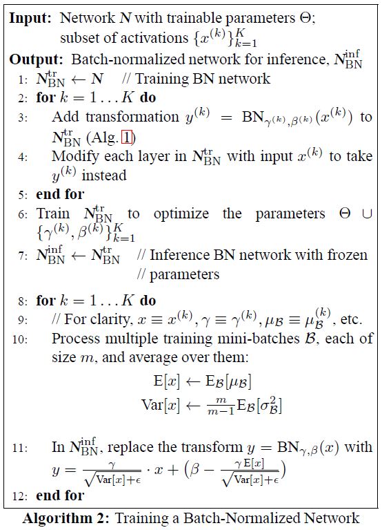
3.1. Training and Inference with Batch-Normalized Networks

To Batch-Normalize a network, we specify a subset of activations and insert the BN transform for each of them, according to Alg.1. Any layer that previously received $x$ as the input, now receives $BN(x)$. A model employing Batch Normalization can be trained using batch gradient descent, or Stochastic Gradient Descent with a mini-batch size $m>1$, or with any of its variants such as Adagrad (Duchi et al., 2011). The normalization of activations that depends on the mini-batch allows efficient training, but is neither necessary nor desirable during inference; we want the output to depend only on the input, deterministically. For this, once the network has been trained, we use the normalization $$\hat{x}=\frac{x-E[x]}{\sqrt{Var[x]+ϵ}}$$ using the population, rather than mini-batch, statistics. Neglecting $ϵ$, these normalized activations have the same mean 0 and variance 1 as during training. We use the unbiased variance estimate $Var[x]=\frac{m}{m-1}\cdot E_B[{\sigma }_{B^2}]$, where the expectation is over training mini-batches of size $m$ and ${\sigma }_{B^2}$ are their sample variances. Using moving averages instead, we can track the accuracy of a model as it trains. Since the means and variances are fixed during inference, the normalization is simply a linear transform applied to each activation. It may further be composed with the scaling by $\gamma$ and shift by $\beta$, to yield a single linear transform that replaces $BN(x)$. Algorithm 2 summarizes the procedure for training batch-normalized networks.

3.1 批标准化网络的训练和推断

为了批标准化一个网络，根据算法1，我们指定一个激活的子集，然后在每一个激活中插入BN变换。任何以前接收$x$作为输入的层现在接收$BN(x)$作为输入。采用批标准化的模型可以使用批梯度下降，或者用小批量数据大小为$m>1$的随机梯度下降，或使用它的任何变种例如Adagrad (Duchi et al., 2011)进行训练。依赖小批量数据的激活值的标准化可以有效地训练，但在推断过程中是不必要的也是不需要的；我们希望输出只确定性地取决于输入。为此，一旦网络训练完成，我们使用总体统计来进行标准化$$\hat{x}=\frac{x-E[x]}{\sqrt{Var[x]+ϵ}}$$，而不是小批量数据统计。跟训练过程中一样，如果忽略$ϵ$，这些标准化的激活具有相同的均值0和方差1。我们使用无偏方差估计$Var[x]=\frac{m}{m-1}\cdot E_B[{\sigma }_B^2]$，其中期望是在大小为$m$的小批量训练数据上得到的，${\sigma }_B^2$是其样本方差。使用这些值移动平均，我们在训练过程中可以跟踪模型的准确性。由于均值和方差在推断时是固定的，因此标准化是应用到每一个激活上的简单线性变换。它可以进一步由缩放$\gamma$和转移$\beta$组成，以产生代替$BN(x)$的单线性变换。算法2总结了训练批标准化网络的过程。

3.2. Batch-Normalized Convolutional Networks

Batch Normalization can be applied to any set of activations in the network. Here, we focus on transforms that consist of an affine transformation followed by an element-wise nonlinearity: $$z=g(Wu+b)$$ where $W$ and $b$ are learned parameters of the model, and $g(\cdot )$ is the nonlinearity such as sigmoid or ReLU. This formulation covers both fully-connected and convolutional layers. We add the BN transform immediately before the nonlinearity, by normalizing $x=Wu+b$. We could have also normalized the layer inputs $u$, but since $u$ is likely the output of another nonlinearity, the shape of its distribution is likely to change during training, and constraining its first and second moments would not eliminate the covariate shift. In contrast, $Wu+b$ is more likely to have a symmetric, non-sparse distribution, that is “more Gaussian” (Hyvärinen & Oja, 2000); normalizing it is likely to produce activations with a stable distribution.

3.2. 批标准化卷积网络

批标准化可以应用于网络的任何激活集合。这里我们专注于仿射变换和元素级非线性组成的变换：$$z=g(Wu+b)$$ 其中$W$和$b$是模型学习的参数，$g(\cdot )$是非线性例如sigmoid或ReLU。这个公式涵盖了全连接层和卷积层。我们在非线性之前通过标准化$x=Wu+b$加入BN变换。我们也可以标准化层输入$u$，但由于$u$可能是另一个非线性的输出，它的分布形状可能在训练过程中改变，并且限制其第一矩或第二矩不能去除协变量转移。相比之下，$Wu+b$更可能具有对称，非稀疏分布，即“更高斯”（Hyvärinen＆Oja，2000）；对其标准化可能产生具有稳定分布的激活。

Note that, since we normalize $Wu+b$, the bias $b$ can be ignored since its effect will be canceled by the subsequent mean subtraction (the role of the bias is subsumed by $\beta$ in Alg.1). Thus, $z=g(Wu+b)$ is replaced with $$z=g(BN(Wu))$$ where the BN transform is applied independently to each dimension of $x=Wu$, with a separate pair of learned parameters ${\gamma }^{(k)}$, ${\beta }^{(k)}$ per dimension.

注意，由于我们对$Wu+b$进行标准化，偏置$b$可以忽略，因为它的效应将会被后面的中心化取消（偏置的作用会归入到算法1的$\beta$）。因此，$z=g(Wu+b)$被$$z=g(BN(Wu))$$替代，其中BN变换独立地应用到$x=Wu$的每一维，每一维具有单独的成对学习参数$\gamma (k)$，$\beta (k)$。

For convolutional layers, we additionally want the normalization to obey the convolutional property —— so that different elements of the same feature map, at different locations, are normalized in the same way. To achieve this, we jointly normalize all the activations in a mini-batch, over all locations. In Alg.1, we let KaTeX parse error: Undefined control sequence: \cal at position 1: \̲c̲a̲l̲ ̲B be the set of all values in a feature map across both the elements of a mini-batch and spatial locations —— so for a mini-batch of size $m$ and feature maps of size $p\times q$, we use the effective mini-batch of size KaTeX parse error: Undefined control sequence: \cal at position 5: m'=|\̲c̲a̲l̲ ̲B| = m\cdot p, …. We learn a pair of parameters ${\gamma }^{(k)}$ and ${\beta }^{(k)}$ per feature map, rather than per activation. Alg.2 is modified similarly, so that during inference the BN transform applies the same linear transformation to each activation in a given feature map.

另外，对于卷积层我们希望标准化遵循卷积特性——为的是同一特征映射的不同元素，在不同的位置，以相同的方式进行标准化。为了实现这个，我们在所有位置联合标准化了小批量数据中的所有激活。在算法1中，我们让$B$是跨越小批量数据的所有元素和空间位置的特征图中所有值的集合——因此对于大小为$m$的小批量数据和大小为$p\times q$的特征映射，我们使用有效的大小为$m^{\prime }=|B|=m\cdot p,q$的小批量数据。我们每个特征映射学习一对参数$\gamma (k)$和$\beta (k)$，而不是每个激活。算法2进行类似的修改，以便推断期间BN变换对在给定的特征映射上的每一个激活应用同样的线性变换。

3.3. Batch Normalization enables higher learning rates

In traditional deep networks, too high a learning rate may result in the gradients that explode or vanish, as well as getting stuck in poor local minima. Batch Normalization helps address these issues. By normalizing activations throughout the network, it prevents small changes in layer parameters from amplifying as the data propagates through a deep network. For example, this enables the sigmoid nonlinearities to more easily stay in their non-saturated regimes, which is crucial for training deep sigmoid networks but has traditionally been hard to accomplish.

3.3. 批标准化可以提高学习率

在传统的深度网络中，学习率过高可能会导致梯度爆炸或梯度消失，以及陷入差的局部最小值。批标准化有助于解决这些问题。通过标准化整个网络的激活值，在数据通过深度网络传播时，它可以防止层参数的微小变化被放大。例如，这使sigmoid非线性更容易保持在它们的非饱和状态，这对训练深度sigmoid网络至关重要，但在传统上很难实现。

Batch Normalization also makes training more resilient to the parameter scale. Normally, large learning rates may increase the scale of layer parameters, which then amplify the gradient during backpropagation and lead to the model explosion. However, with Batch Normalization, backpropagation through a layer is unaffected by the scale of its parameters. Indeed, for a scalar $a$, $$BN(Wu)=BN((aW)u)$$ and thus $\frac{\partial BN((aW)u)}{\partial u}=\frac{\partial BN(Wu)}{\partial u}$, so the scale does not affect the layer Jacobian nor, consequently, the gradient propagation. Moreover, $\frac{\partial BN((aW)u)}{\partial (aW)}=\frac{\partial BN(Wu)}{\partial W}$ so larger weights lead to smaller gradients, and Batch Normalization will stabilize the parameter growth.

批标准化也使训练对参数的缩放更有弹性。通常，大的学习率可能会增加层参数的缩放，这会在反向传播中放大梯度并导致模型爆炸。然而，通过批标准化，通过层的反向传播不受其参数缩放的影响。实际上，对于标量$a$，$$BN(Wu)=BN((aW)u)$$因此$\frac{\partial BN((aW)u)}{\partial u}=\frac{\partial BN(Wu)}{\partial u}$，因此标量不影响层的雅可比行列式，从而不影响梯度传播。此外，$\frac{\partial BN((aW)u)}{\partial (aW)}=\frac{1}{a}\cdot \frac{\partial BN(Wu)}{\partial W}$，因此更大的权重会导致更小的梯度，并且批标准化会稳定参数的增长。

We further conjecture that Batch Normalization may lead the layer Jacobians to have singular values close to 1, which is known to be beneficial for training (Saxe et al., 2013). Consider two consecutive layers with normalized inputs, and the transformation between these normalized vectors: $\hat{z}=F(\hat{x})$. If we assume that $\hat{x}$ and $\hat{z}$ are Gaussian and uncorrelated, and that $F(\hat{x})\approx J\hat{x}$ is a linear transformation for the given model parameters, then both $\hat{x}$ and $\hat{z}$ have unit covariances, and $I=Cov[\hat{z}]=JCov[\hat{x}]J^T=J{J}^T$. Thus, $J$ is orthogonal, which preserves the gradient magnitudes during backpropagation. Although the above assumptions are not true in reality, we expect Batch Normalization to help make gradient propagation better behaved. This remains an area of further study.

我们进一步推测，批标准化可能会导致雅可比行列式的奇异值接近于1，这被认为对训练是有利的(Saxe et al., 2013)。考虑具有标准化输入的两个连续的层，并且变换位于这些标准化向量之间：$\hat{z}=F(\hat{x})$。如果我们假设$\hat{x}$和$\hat{z}$是高斯分布且不相关的，那么$F(\hat{x})\approx J\hat{x}$是对给定模型参数的一个线性变换，$\hat{x}$和$\hat{z}$有单位方差，并且$I=Cov[\hat{z}]=JCov[\hat{x}]J^T=J{J}^T$。因此，$J$是正交的，其保留了反向传播中的梯度大小。尽管上述假设在现实中不是真实的，但我们希望批标准化有助于梯度传播更好的执行。这有待于进一步研究。