


TensorFlow 2.0 入门实战笔记(持续更新)
一、初见Tensorflow
1.1 2015年之前的深度学习框架:
- Scikit-learn
- Machine learning, No GPU
- Caffe
- 2013, 第一个面向深度学习的框架
- No auto-grad, C++
- Keras
- wrapper
- Theano
- 开发难,调试难
- Torch
- Lua语言
1.2 深度学习框架发展
- Caffe
▪ Facebook,Caffe2 → PyTorch
▪ Torch → PyTorch - Theano
▪ Google, → TensorFlow
▪ → TensorFlow 2
从今天开始,忘掉TensorFlow 1.x
1.3 2015年之后TF版本:
- 2015.9发布0.1版本
- 2017.2发布1.0版本
- 2019春发布2.0版本
- 直到现在(2020/4/28)2.1 稳定版
1.4 安装TF
默认安装GPU版
pip install tensorflow
具体是CUDA和cuDNN可以暂时参考TensorFlow2.1.0安装教程
安装完成后的测试参考tensorflow-gpu-2.1安装成功测试代码
1.5 Pycharm关闭红色字体日志输出
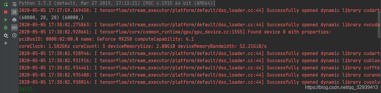
关闭以上[令人讨厌的]红色字体日志输出的方法如下:
在import tensorflow as tf之前添加os.environ['TF_CPP_MIN_LOG_LEVEL'] = '2',必须是之前,否则无效,鬼知道为什么
import os
os.environ['TF_CPP_MIN_LOG_LEVEL'] = '2'
import tensorflow as tf
二、Tensorflow基础操作
2.1 数据类型
- 标量:单个实数,维度(秩)为0,shape为 [ ]
- 向量:n个实数的有序集合,秩为1,shape为[n]
- 矩阵:n行m列的有序集合,秩为2,shape为[n, m]
- 张量:所有维度数 dim > 2 的数组统称为张量,张量的每个维度也叫做轴(axis)
在tensorflow中,一般也把标量、向量、矩阵也统称为张量,不作区分。
2.1.1 数据载体
list支持不同的数据类型,效率低
np.array相同类型的载体,效率高,但是不支持GPU,不支持自动求导
tf.Tensortensorflow中存储大量连续数据的载体
2.1.2 基本数据类型
tf.int32:tf.constant(1)
tf.float32:tf.constant(1.)
tf.float64: tf.constant(1., dtype=tf.double)
tf.bool: tf.constant([True, False])
tf.string:tf.constant('hello')
2.1.3 数值精度
常用的数值精度有:tf.int16, tf.int32, tf.int64, tf.float16, tf.float32, tf.float64, 其中tf.float64即为tf.double
可通过dtype设置数值精度
In [10]: tf.constant(2, dtype = tf.double)
Out[10]: <tf.Tensor: id=8, shape=(), dtype=float64, numpy=2.0>
2.1.4 数据基本属性
with tf.device("cpu"):
    a=tf.range(4)
a.device # '/job:localhost/replica:0/task:0/device:CPU:0'
aa=a.gpu()
a.numpy() # array([0, 1, 2, 3], dtype=int32) [转换为numpy格式]
a.ndim # 1  (0的话就是标量) [显示当前维度,返回一个标量]
a.shape # TensorShape([4]) [返回张量的形状]
a.name # AttributeError: Tensor.name is meaningless when eager execution is enabled.
tf.rank(tf.ones([3,4,2])) # <tf.Tensor: id=466672, shape=(), dtype=int32, numpy=3>[显示当前维度,返回一个张量]
tf.is_tensor(a) # True [判断是否为Tensor类型,返回True/False]
a.dtype # tf.int32 [返回数据类型]
device:显示当前设备
a.gpu()/ a.cpu:设备的切换
rank和ndim的区别在于返回的类型不同
name属性在tensorflow2没有意义,因为变量名本身就是name
2.1.4 Array 和 Tensor的不同之处:
判断一个变量究竟是tensor还是array,直接输出它的dtype,输出上面那样的就是tensor,输出下面那样的就是array
输入
a=tf.constant([[1,2],[3,4]],dtype=tf.float32)
print(a.dtype)
b=np.array([[1,2],[3,4]],dtype='float32')
print(b.dtype)

输出:
<dtype: 'float32'>
float32
2.1.5 Array 和 Tensor的转换:
Numpy中的存储格式为Array
a=np.arange(5) # [0, 1, 2, 3, 4]
a.dtype # dtype('int64')
aa=tf.convert_to_tensor(a) # <tf.Tensor: id=466678, shape=(5,), dtype=int64, numpy=array([0, 1, 2, 3, 4])>[将aa转换为tensor]
aa=tf.convert_to_tensor(a, dtype=tf.int32) # <tf.Tensor: id=466683, shape=(5,), dtype=int32, numpy=array([0, 1, 2, 3, 4], dtype=int32)>[将aa转换为tensor类型的同时指定dtype]
tf.cast(aa, tf.float32) # 将aa 转换为 float32类型

b=tf.constant([0,1])
tf.cast(b, tf.bool) # <tf.Tensor: id=466697, shape=(2,), dtype=bool, numpy=array([False,  True])>

a.tf.ones([2,3])
a.numpy()# [将a转换为Array]
int(a) #标量可以直接这样类型转换
float(a)
2.1.6 可训练数据类型:
只有Variable类型的张量可以通过训练自动改变值
a=tf.range(5)
b=tf.Variable(a)
b.dtype # tf.int32
b.name # 'Variable:0' 其实没啥用
b.trainable #True 可训练
2.2 创建Tensor
tf.convert_to_tensor(data) 将data转换为tensor,其中data 可以为np.ones(shape)、np.zeros(shape) 、[1,2]等numpy矩阵
tf.zeros(shape)生成一个tensor,维度形状为shape
tf.ones(1)生成一个一维tensor,包含一个1
tf.ones([])生成一个标量1
tf.ones([2])生成一个一维tensor,包含两个1
tf.ones_like(a)相当于tf.ones(a.shape)
tf.fill([3,4], 9) 全部填充9
tf.random.normal([3,4], mean=1, stddev=1) 正态分布随机生成,形状为(3,4)mean 均值 ,stddev 标准差
tf.random.truncated_normal([3,4], mean=0, stddev=1) 带截断的正态分布,(大于某个值重新采样),比如在经过sigmoid激活后,如果用带截断的,可以避免出现梯度消失问题。
tf.random.uniform([3,4], minval=0, maxval=100, dtype=tf.int32)平均分布
tf.constant(a)a为常量或定值Tensor
idx=tf.random.shuffle(idx)#随机打散idx
令a,b有对应关系,则a,b打散之后仍有对应关系
idx=tf.range(5)
idx=tf.random.shuffle(idx) # 随机打散idx
a=tf.random.normal([10,784])
b=tf.random.uniform([10])
a=tf.gather(a, idx) # a中随机取5行
b=tf.gather(b, idx) # b中随机取5个
2.3 索引与切片
2.3.1 索引
基本:a[idx][idx][idx],a为Tensor
In [4]:a=tf. ones([1,5,5,3])
In [5]:a[0][0]
<tf. Tensor: id=16, shape=(5,3), dtype=float32, numpy=
array([ [1.,1.,1.],
		[1.,1.,1.],
		[1.,1.,1.],
		[1.,1.,1.],
		[1.,1.,1.]], dtype=float32)>
In [6]:a[0][0][0]
Out[6]:<tf. Tensor: id=29, shape=(3,), dtype=float32, numpy=array([1.,1.,1.], dtype=float32)>
In [7]:a[0][0][0][2]
0ut[7]:<tf. Tensor: id=46, shape=(), dtype=float32, numpy=1.0>
numpy风格:a[idx,idx,idx]可读性更强
In [8]:a=tf. random. normal([4,28,28,3])
In [9]:a[1]. shape
Out[9]: TensorShape([28,28,3])
In [10]:a[1,2]. shape
Out[10]: TensorShape([28,3])
In [11]:a[1,2,3]. shape
Out[11]: TensorShape([3])
In [12]:a[1,2,3,2]. shape
Out[12]: TensorShape([])
2.3.2 一般切片
与numpy基本一致
a[start:end:positive_step]
a[end:start:negative_step]
a[0, 1, ..., 0]代表任意多个: 只要能推断出有多少个:就是合法的
[A:B]表示从A位置取到B位置,A位置包含在内,B位置不包含在内
[A: ]从A位置去到末尾位置
[ :B]从起始0位置取到B位置,但不包含B位置
[ : ]从起始位置到末尾位置,取遍所有
Start:End
In [8]:a=tf. range(10)
Out[9]:<tf. Tensor: numpy=array([o,1,2,3,4,5,6,7,8,9])>
In [14]:a[-1:]
Out[14]:<tf. Tensor: id=48, shape=(1,), dtype=int32, numpy=array([9])>
In [15]:a[-2:]
Out[15]:<tf. Tensor: id=53, shape=(2,), dtype=int32, numpy=array([8,9])>
In [16]:a[:2]
Out[16]:<tf. Tensor: id=58, shape=(2,), dtype=int32, numpy=array([o,1])>
In [17]:a[:-1]
Out[17]:<tf. Tensor: id=63, shape=(9,), dtype=int32, numpy=array([o,1,2,3,4,
5,6,7,8])>
In [14]:a. shape # TensorShape([4,28,28,3])
In [15]:a[0]. shape # TensorShape([28,28,3])
In [16]:a[0,:,:,:]. shape
0ut[16]: TensorShape([28,28,3])
In[17]:a[0,1,:,:]. shape
0ut[17]: TensorShape([28,3])
In [18]:a[:,:,:,0]. shape
0ut[18]: TensorShape([4,28,28])
In [19]:a[:,:,:,2]. shape
0ut[19]: TensorShape([4,28,28])
In [20]:a[:,0,:,:]. shape
0ut[20]: TensorShape([4,28,3])
[A:B:N]表示从A位置到B位置,每隔N个位置取一次,A位置包含在内,B位置不包含在内,
Start:End:Step
In [21]:a. shape
Out[21]: TensorShape([4,28,28,3])
In [22]:a[0:2,:,:,:]. shape
Out[22]: TensorShape([2,28,28,3])
In [23]: al:,0:28:2,0:28:2,:]. shape
Out[23]: TensorShape([4,14,14,3])
In [24]:a[:,:14,:14,:]. shape
Out[24]: TensorShape([4,14,14,3])
In [25]:a[:,14:,14:,:]. shape
0ut[25]: TensorShape([4,14,14,3])
In [26]: al:,::2,::2,:]. shape
Out[26]: TensorShape([4,14,14,3])
Step还可以为负值
In [27]:a=tf. range(4)
Out[28]:<tf. Tensor: id=118, shape=(4,), dtype=int32, numpy=array([o,1,2,3], dtype=int32)>
In [29]:a[::-1]
Out[29]:<tf. Tensor: id=123, shape=(4,), dtype=int32, numpy=array([3,2,1,0], dtype=int32)>
In [30]:a[::-2]
Out[30]:<tf. Tensor: id=128, shape=(2,), dtype=int32, numpy=array([3,1], dtype=int32)>
In [31]:a[2::-2]
out[31]:<tf. Tensor: id=133, shape=(2,), dtype=int32, numpy=array([2,0], dtype=int32)>
"···" 表示系统自动推断剩余维度
In [36]:a=tf. random. normal([2,4,28,28,3])
In [37]:a[0]. shape
Out[37]: TensorShape([4,28,28,3])
In [38]:a[0,:,:,:,:]. shape
Out[38]: TensorShape([4,28,28,3])
In [39]:a[0,...]. shape
Out[39]: TensorShape([4,28,28,3])
In [40]:a[:,:,:,:,0]. shape
Out[40]: TensorShape([2,4,28,28])
In [41]:a[...,0]. shape
Out[41]: TensorShape([2,4,28,28])
In [42]:a[0,...,2]. shape
Out[42]: TensorShape([4,28,28])
In [43]:a[1,0,...,0]. shape
Out[43]: TensorShape([28,28])
2.3.3 Selective Indexing
tf.gather(params,,axis ,indices)
其中params为张量,axis为维度轴,indices表示从此维度选取的元素并且重排为设定顺序,
场景:
假设每个维度的意义:data: [classes, students, subjects]
[4, 35, 8] 代表有4个classes,每个class有35个student,每个学生学习8个subject
# a[4,35,8]
In [46]: tf.gather(a, axis=0, indices=[2,3]).,shape #axis=0表示按照classes维度取
								# indices=[2,3]表从4个班级中选取第二个和第三个班级顺序按照2,3
Out[46]: TensorShape([2,35,8])
In [47]:a[2:4]. shape
Out[47]: Tensor Shape([2,35,8])
In [48]: tf. gather(a, axis=0, indices=[2,1,4,0]). shape # indices=[2,1,4,0]取到的班级顺序按照2,1,4,0 重排顺序
Out[48]: TensorShape([4,35,8])
In [49]: tf. gather(a, axis=1, indices=[2,3,7,9,16]). shape
Out[49]: TensorShape([4,5,8])
In [50]: tf. gather(a, axis=2, indices=[2,3,7]). shape
Out[50]: TensorShape([4,35,3])
tf.gather_nd( params, indices, name=None)
W3Cshool解释
类比tf.gather可同时制定多个维度进行选择切片
In [55]:a. shape Out[55]: Tensor Shape([4,35,8])
In [60]: tf. gather_nd(a,[0]). shape
Out[60]: TensorShape([35,8])
In [61]: tf. gather_nd(a,[0,1]). shape
Out[61]: TensorShape([8])
In [62]: tf. gather_nd(a,[o,1,2]). shape
Out[62]: TensorShape([])
In [63]: tf. gather_nd(a,[[o,1,2]]). shape
Out[63]: TensorShape([1])
In [55]:a. shape Out[55]: TensorShape([4,35,8])
In [56]: tf. gather_nd(a,[[o,0],[1,1]]). shape
Out[56]: Tensor Shape([2,8])
In [57]: tf. gather_nd(a,[[0,0],[1,1],[2,2]]). shape
Out[57]: TensorShape([3,8])
In [58]: tf. gather_nd(a,[[o,0,0],[1,1,1],[2,2,2]]). shape
Out[58]: Tensor Shape([3])
In [59]: tf. gather_nd(a,[[[0,0,0],[1,1,1],[2,2,2]]]). shape
Out[59]: TensorShape([1,3])
tf.boolean_mask
tf.boolean_mask(a, mask=[True, True, False], axis=3)axis=3是第四维度表RGB, 相当于只取3个通道中的前两个RG的数据, a的shape是[4, 28, 28, 3]。mask可以是一个list。
In[75]:a. shape
Out[75]: TensorShape([4,28,28,3])
In [76]: tf. boolean_mask(a, mask=[ True, True, False, False]). shape
0ut[76]: Tensor Shape([2,28,28,3])
In [77]: tf. boolean_mask(a, mask=[ True, True, False], axis=3). shape
Out[77]: TensorShape([4,28,28,2])
In [78]:a=tf. ones([2,3,4])
In [79]: tf. boolean_mask(a, mask=[[ True, False, False],[ False, True, True]])
<tf. Tensor: id=354, shape=(3,4), dtype=float32, numpy=
array([ [1.,1.,1.,1.],
		[1.,1.,1.,1.],
		[1.,1.,1.,1.J], dtype=float32)>
2.4 维度变换
- 查看形状
a.shape - 查看当前维度
a.ndim
2.4.1 图片的存储View
- [b, 28, 28] 考虑行和列
- →[b, 28*28] 不考虑行和列,神经网络全连接的View方式
- →[b, 2, 14*28] 图片存储为上下两部分
- →[b, 28, 28, 1] 加入channel概念,1可省略
2.4.2 tf.transpose 交换图像的行列【转置】
a=tf.random.normal([4, 3, 2, 1])
tf.transpose(a, perm=[0, 1, 3, 2])# 0,1不变,相当于交换最后两维
# 输出为 [4,3,1,2]
2.4.2 tf.reshape 重置维度
Reshape可提供无数种重置形状的可能,但并非都可解释,或者说属性都有物理意义
Reshape要保证所有pixel数量不变
In [80]:a=tf. random. normal([4,28,28,3])
Out[81]: TensorShape([4,28,28,3])
In [82]:a. shape,a. ndim
0ut[82]:(Tensor Shape([4,28,28,3]),4)
In [83]: tf. reshape(a,[4,784,3]). shape
Out[83]: TensorShape([4,784,3])
In [84]: tf. reshape(a,[4,-1,3]). shape
Out[84]: TensorShape([4,784,3])
In [85]: tf. reshape(a,[4,784*3]). shape
Out[85]: TensorShape([4,2352])
In [86]: tf. reshape(a,[4,-1]). shape
Out[86]: TensorShape([4,2352])
2.4.3 tf.expand_dims增加维度
dim和axis含义类似
a=tf.random.normal([4, 35, 8])
tf.expand_dims(a, axis=3)  # 增加的维度是第4(3+1)维 shape是[4, 35, 8, 1]
tf.expand_dims(a, axis=0)  # 增加的维度是第 0 维 shape是[ 1,4, 35, 8]
axis 指的是扩展维度轴的位置
In [103]:a=tf. random. normal([4,35,8])
In [105]: tf. expand_dims(a, axis=0). shape
Out[105]: TensorShape([1,4,35,8])
In [106]: tf. expand_dims(a, axis=3). shape
Out[106]: TensorShape([4,35,8,1])
In [107]: tf. expand_dims(a, axis=-1). shape
Out[107]: Tensor Shape([4,35,8,1])
In [108]: tf. expand_dims(a, axis=-4). shape
Out[108]: TensorShape([1,4,35,8])
2.4.4 tf.squeeze 压缩维度
默认去掉所有长度是1的维度,也可以通过axis指定某一个维度
In [115]: tf. squeeze(tf. zeros([1,2,1,1,3])). shape
Out[115]: TensorShape([2,3])
In [116]:a=tf. zeros([1,2,1,3])
In [117]: tf. squeeze(a, axis=0). shape
Out[117]: TensorShape([2,1,3])
In [118]: tf. squeeze(a, axis=2). shape
Out[118]: TensorShape([1,2,3])
In [119]: tf. squeeze(a, axis=-2). shape
Out[119]: TensorShape([1,2,3])
In [120]: tf. squeeze(a, axis=-4). shape
Out[120]: TensorShape([2,1,3])
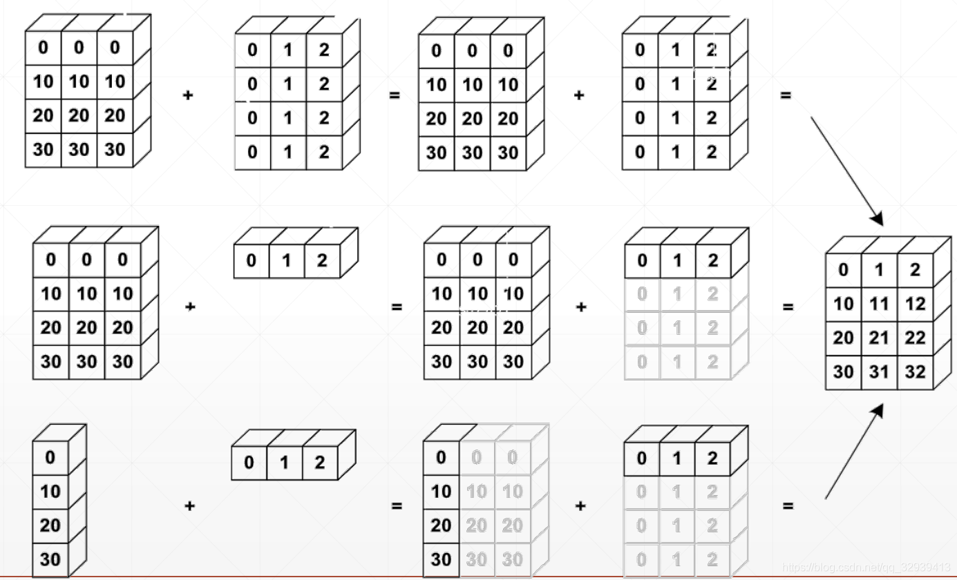
2.5 Broadcasting
若相加的两个Tensor的维度不一致,则扩展其中一个Tensor的维度与另一个对齐,但内存中并未发生数据复制;
原则:低维度对齐,低维度不同则不同
在实际使用的过程中往往可省略,由解释器自动判断完成
tf. broadcast_to
场景:一般情况下,高维度比低维度的概念更高层,如[班级,学生,成绩],利用broadcasting把小维度推广到大维度。
作用:简洁、节省内存
In [35]:x. shape Out[35]: TensorShape([4,32,32,3])
In [36]:(x+tf. random. normal([4,1,1,1])). shape
Out[36]: TensorShape([4,32,32,3])
In [37]:b=tf. broadcast_to(tf. random. normal([4,1,1,1]),[4,32,32,3])
In [38]:b. shape
Out[38]: Tensor Shape([4,32,32,3])
参考:https://www.cnblogs.com/chenhuabin/p/11594239.html#_label3
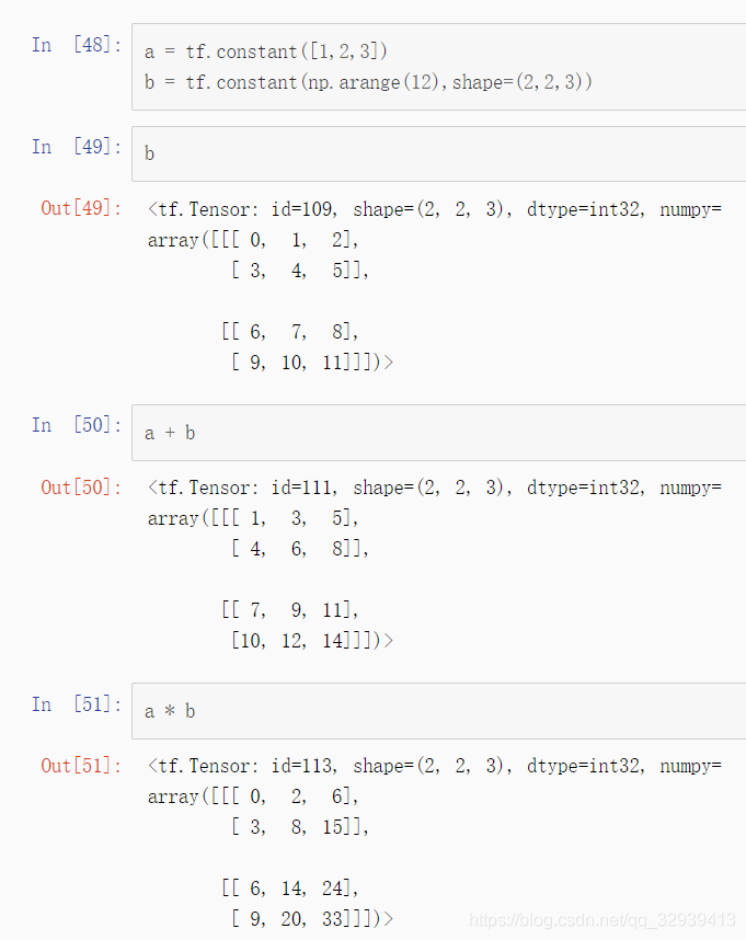
可以看到,一个一维的张量与一个三维张量进行运算是完全没有问题的,从运算结果上可以看出,相当于是三维张量中的每一行数据与张量a进行运算,为什么可以这样运输呢?这就得益于TensorFlow中的Broadcasting机制。Broadcasting机制解除了只能维度数和形状相同的张量才能进行运算的限制,当两个数组进行算术运算时,TensorFlow的Broadcasting机制首先对维度较低的张量形状数组填充1,从后向前,逐元素比较两个数组的形状,当逐个比较的元素值(注意,这个元素值是指描述张量形状数组的值,不是张量的值)满足以下条件时,认为满足
Broadcasting 的条件:(1)相等
(2)其中一个张量形状数组元素值为1。
当不满足时进行运算则会抛出 ValueError: frames are not aligne
异常。算术运算的结果的形状的每一元素,是两个数组形状逐元素比较时的最大值。回到上面张量a与b相乘的例子,a的形状是(3,),b的形状是(2, 2,
3),在Broadcasting机制工作时,首先比较维度数,因为a的维度为1,小于b的维度3,所以填充1,a的形状就变成了(1,1,3),然后从最后端的形状数组元素依次往前比较,先是就是3与3比,结果是相等,接着1与2相比,因为其中一个为1,所以a的形状变成了(1,2,3),继续1与2比较,因为其中一个为1,所以a的形状变成了(2,2,3),a中的数据每一行都填充a原来的数据,也就是[1,2,3],然后在与b进行运算。当然,在TensorFlow的Broadcasting机制运行过程中,上述操作只是理论的,并不会真正的将a的形状变成(2,2,3,),更不会将每一行填充[1,2,3],只是虚拟进行操作,真正计算时,依旧是使用原来的张量a。这么做的好处是运算效率更高,也更节省内存。
Broadcast VS Tile(复制)
In [4]:a=tf. ones([3,4])
In [5]: al=tf. broadcast_to(a,[2,3,4])
<tf. Tensor: id=7, shape=(2,3,4), dtype=float32, numpy=
arrayC[[[4.,1.,1.,1.],
		[4.,1.,1.,1.],
		[4.,1.,1.,1.]],

		[[4.,1.,1.,1.],
		[4.,1.,1.,1.],
		[1.,1.,1.,1.]]], dtype=float32)>
In [7]:a2=tf. expand_dims(a, axis=0)
0ut[8]: TensorShape([1,3,4])
In [40]:a2=tf. tile(a2,[2,1,1])
<tf. Tensor: id=12, shape=(2,3,4), dtype=float32, annpyf[[[4.,1.,1.,1.],
														[4.,1.,1.,1.],
														[4.,1.,1.,1.]],

														[[4.,1.,1.,1.],
														[4.,1.,1.,1.],
														[4.,1.,1.,1.]]], dtupe=float32)>
2.6 数学运算
常用的数学运算
可参考【tensorflow 2.0 基础操作 之 数学运算】
+ - * / // %
tf.math.log && tf.exp
pow , sqrt
@ tf.matmul
liner layer
2.6.1 + - * / // %运算
+:对应矩阵元素相加
-:对应矩阵元素相减
*:对应矩阵元素相除
/:对应矩阵元素相除
%:对应矩阵元素求余
//:对应矩阵元素整除
/除法计算结果是浮点数,即使是两个整数恰好整除,结果也是浮点数;
//,称为地板除,两个整数的除法仍然是整数。
基本运算中所有实例都以下面的张量a、b为例进行:
In [2]: a = tf.ones([2,2])#2*2矩阵,全部填充为1

In [3]: b =  tf.fill([2,2],2.)#2*2矩阵,全部填充为2

In [4]: a
Out[4]:
<tf.Tensor: id=2, shape=(2, 2), dtype=float32, numpy=
array([[1., 1.],
       [1., 1.]], dtype=float32)>

In [5]: b
Out[5]:
<tf.Tensor: id=5, shape=(2, 2), dtype=float32, numpy=
array([[2., 2.],
       [2., 2.]], dtype=float32)>

In [6]: a + b#对应矩阵元素相加
Out[6]:
<tf.Tensor: id=8, shape=(2, 2), dtype=float32, numpy=
array([[3., 3.],
       [3., 3.]], dtype=float32)>

In [7]: a - b#对应矩阵元素相减
Out[7]:
<tf.Tensor: id=10, shape=(2, 2), dtype=float32, numpy=
array([[-1., -1.],
       [-1., -1.]], dtype=float32)>

In [8]: a * b #对应矩阵元素相乘
Out[8]:
<tf.Tensor: id=12, shape=(2, 2), dtype=float32, numpy=
array([[2., 2.],
       [2., 2.]], dtype=float32)>

In [9]: a / b#对应矩阵元素相除
Out[9]:
<tf.Tensor: id=14, shape=(2, 2), dtype=float32, numpy=
array([[0.5, 0.5],
       [0.5, 0.5]], dtype=float32)>

In [10]: b // a #对应矩阵元素整除
Out[10]:
<tf.Tensor: id=16, shape=(2, 2), dtype=float32, numpy=
array([[2., 2.],
       [2., 2.]], dtype=float32)>

In [11]: b % a #对应矩阵元素求余
Out[11]:
<tf.Tensor: id=18, shape=(2, 2), dtype=float32, numpy=
array([[0., 0.],
       [0., 0.]], dtype=float32)>
可以看出,对于基本运算加(+)、减(-)、点乘(*)、除(/)、地板除法(//)、取余(%),都是对应元素进行运算。
2.6.2 tf.math.log( ) 和tf.math.exp( ) 函数
tf.math.log( )以e为底求对数
tf.math.exp( n )e的n次方
In [12]: a = tf.ones([2,2])

In [13]: a
Out[13]:
<tf.Tensor: id=22, shape=(2, 2), dtype=float32, numpy=
array([[1., 1.],
       [1., 1.]], dtype=float32)>

In [14]: tf.math.log(a)#矩阵对应元素取对数
Out[14]:
<tf.Tensor: id=24, shape=(2, 2), dtype=float32, numpy=
array([[0., 0.],
       [0., 0.]], dtype=float32)>

In [15]: tf.math.exp(a)#矩阵对应元素取指数
Out[15]:
<tf.Tensor: id=26, shape=(2, 2), dtype=float32, numpy=
array([[2.7182817, 2.7182817],
       [2.7182817, 2.7182817]], dtype=float32)>
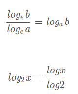
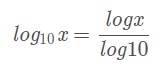
log 但是 没有以其他 为底的 API
实现 以2,10 为底
In [17]: a = tf.random.normal([2,2])

In [18]: a
Out[18]:
<tf.Tensor: id=38, shape=(2, 2), dtype=float32, numpy=
array([[ 0.12121297, -1.6076226 ],
       [ 1.4407614 ,  0.8430799 ]], dtype=float32)>

In [19]: tf.math.log(a)/tf.math.log(2.)#计算矩阵对应元素以2为底的对数
Out[19]:
<tf.Tensor: id=43, shape=(2, 2), dtype=float32, numpy=
array([[-3.044384  ,         nan],
       [ 0.5268315 , -0.24625869]], dtype=float32)>

In [20]: tf.math.log(a)/tf.math.log(10.)#计算矩阵对应元素以10为底的对数
Out[20]:
<tf.Tensor: id=48, shape=(2, 2), dtype=float32, numpy=
array([[-0.91645086,         nan],
       [ 0.15859208, -0.07413125]], dtype=float32)>
参考 : https://blog.csdn.net/z_feng12489/article/details/89341002
2.6.3 tf.pow( )和 tf.sqrt( )函数
tf.pow(a,3)矩阵a所有元素取立方
a**3矩阵a所有元素取立方
tf.sqrt(a)矩阵a所有元素开平方
In [2]: a = tf.fill([2,2],2.)

In [3]: a
Out[3]:
<tf.Tensor: id=2, shape=(2, 2), dtype=float32, numpy=
array([[2., 2.],
       [2., 2.]], dtype=float32)>

In [4]: tf.pow(a,3)#矩阵a所有元素取立方
Out[4]:
<tf.Tensor: id=5, shape=(2, 2), dtype=float32, numpy=
array([[8., 8.],
       [8., 8.]], dtype=float32)>

In [5]: a**3#矩阵a所有元素取立方
Out[5]:
<tf.Tensor: id=8, shape=(2, 2), dtype=float32, numpy=
array([[8., 8.],
       [8., 8.]], dtype=float32)>

In [6]: tf.sqrt(a)#矩阵a所有元素开平方
Out[6]:
<tf.Tensor: id=10, shape=(2, 2), dtype=float32, numpy=
array([[1.4142135, 1.4142135],
       [1.4142135, 1.4142135]], dtype=float32)>
2.6.4 @ matmul 矩阵相乘
@与matmul等价作用
In [7]: a = tf.fill([2,2],1.)

In [8]: b = tf.fill([2,2],2.)

In [9]: a,b
Out[9]:
(<tf.Tensor: id=14, shape=(2, 2), dtype=float32, numpy=
 array([[1., 1.],
        [1., 1.]], dtype=float32)>,
 <tf.Tensor: id=17, shape=(2, 2), dtype=float32, numpy=
 array([[2., 2.],
        [2., 2.]], dtype=float32)>)

In [10]: a @ b#矩阵相乘
Out[10]:
<tf.Tensor: id=20, shape=(2, 2), dtype=float32, numpy=
array([[4., 4.],
       [4., 4.]], dtype=float32)>

In [11]: tf.matmul(a,b)#矩阵相乘
Out[11]:
<tf.Tensor: id=22, shape=(2, 2), dtype=float32, numpy=
array([[4., 4.],
       [4., 4.]], dtype=float32)>
In [12]: a = tf.ones([4,2,3])

In [13]: b = tf.fill([4,3,5],2.)

In [14]: a@b    #[2,3]@[3,5] = [2,5]
Out[14]:
<tf.Tensor: id=30, shape=(4, 2, 5), dtype=float32, numpy=
array([[[6., 6., 6., 6., 6.],
        [6., 6., 6., 6., 6.]],

       [[6., 6., 6., 6., 6.],
        [6., 6., 6., 6., 6.]],

       [[6., 6., 6., 6., 6.],
        [6., 6., 6., 6., 6.]],

       [[6., 6., 6., 6., 6.],
        [6., 6., 6., 6., 6.]]], dtype=float32)>

In [15]: tf.matmul(a,b)
Out[15]:
<tf.Tensor: id=32, shape=(4, 2, 5), dtype=float32, numpy=
array([[[6., 6., 6., 6., 6.],
        [6., 6., 6., 6., 6.]],

       [[6., 6., 6., 6., 6.],
        [6., 6., 6., 6., 6.]],

       [[6., 6., 6., 6., 6.],
        [6., 6., 6., 6., 6.]],

       [[6., 6., 6., 6., 6.],
        [6., 6., 6., 6., 6.]]], dtype=float32)>
With broadcasting
In [164]:a. shape # TensorShape([4,2,3])
In [165]:b. shape # TensorShape([3,5])
In [166]: bb=tf. broadcast_to(b,[4,3,5])
In [167]: adbb
<tf. Tensor: id=516, shape=(4,2,5), dtype=float32, numpy=
array([[[6.,6.,6.,6.,6.],
[6.,6.,6.,6.,6.]],..
[[6.,6.,6.,6.,6.],
[6.,6.,6.,6.,6.]]], dtype=f loat32)>
2.6.5 liner layer
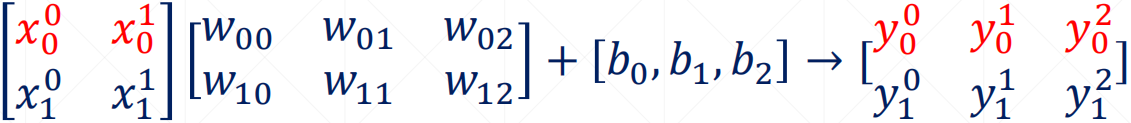
参考 : https://blog.csdn.net/z_feng12489/article/details/89341002
𝑍 = 𝑌@𝑋 + 𝑏
In [168]:x=tf. ones([4,2]) In [169]:W=tf. ones([2,1])
In [170]:b=tf. constant(0.1)
In [171]: xCW+b
<tf. Tensor: id=526, shape=(4,1), dtype=float32, numpy=
array([[2.1],
[2.1],[2.1],
[2.1]], dtype=float32)>
out = relu(𝑌@𝑋 + 𝑏)
In [171]:x@W+b
<tf. Tensor: id=526, shape=(4,1), dtype=float32, numpy=
array([[2.1],
[2.1],[2.1],
[2.1]], dtype=float32)>
In [172]: out=x@W+b In [173]: out=tf. nn. relu(out)
<tf. Tensor: id=530, shape=(4,1), dtype=float32, numpy=
array([[2.1],
[2.1],[2.1],
[2.1]], dtype=float32)>
2.6.6 运算类型
element-wise (元素相关)
- + - * \
matrix-wise (矩阵相关)
- @ matmul
dim-wise (维度相关)
- reduce_mean/max/min/sum
reduce_mean获得所有元素的均值
max/min 获得最大/小值元素
sum求和
2.6.7 范数

ord:指定p范数
import tensorflow as tf
a = tf.constant([[1.,2.],[1.,2.]])
tf.norm(a, ord=1)  # 1范数
<tf.Tensor: id=4, shape=(), dtype=float32, numpy=6.0>
tf.norm(a, ord=2)  # 2范数
<tf.Tensor: id=10, shape=(), dtype=float32, numpy=3.1622777>
tf.norm(a)  # ord不指定时,默认是2
<tf.Tensor: id=16, shape=(), dtype=float32, numpy=3.1622777>
我们也可以全手动地实现范数:
tf.sqrt(tf.reduce_sum(tf.square(a)))
<tf.Tensor: id=21, shape=(), dtype=float32, numpy=3.1622777>
# 指定维度求范数:

tf.norm(a, ord=2, axis=0)
<tf.Tensor: id=27, shape=(2,), dtype=float32, numpy=array([1.4142135, 2.828427 ], dtype=float32)>
tf.norm(a, ord=2, axis=1)
<tf.Tensor: id=33, shape=(2,), dtype=float32, numpy=array([2.236068, 2.236068], dtype=float32)>
参考:https://mp.weixin.qq.com/s?__biz=MzA4MjYwMTc5Nw%3D%3D&chksm=87941340b0e39a56e667ba54d9ef8897c41ceaa6ec8be4bacfd77a45743ee27a4db76cd8b7a1&idx=2&mid=2648932714&scene=21&sn=500485be159da8635016331dbbbb5e32#wechat_redirect
三、Tensorflow高阶操作
3.1 合并与分割
3.1.1 tf.concat([a, b], axis) 拼接
tf.concat([a, b], axis)合并,在原来的维度上累加,axis维度合并,要求其他维度的长度都相等
In [8]:a=tf. ones([4,32,8])
In [9]:b=tf. ones([4,3,8])
In [10]: tf. concat([a,b], axis=1). shape
Out[10]: TensorShape([4,35,8])
3.1.2 tf.stack([a, b], axis) 堆叠
tf.stack([a, b], axis)堆叠,axis维度合并,要求所有维度的长度都相等
In [19]:a. shape Out[19]: TensorShape([4,35,8])
In [23]:b. shape Out[23]: Tensor Shape([4,35,8])
In [20]: tf. concat([a,b], axis=-1). shape
Out[20]: Tensor Shape([4,35,16])
In [21]: tf. stack([a,b], axis=0). shape
Out[21]: Tensor Shape([2,4,35,8])
In [22]: tf. stack([a,b], axis=3). shape
Out[22]: TensorShape([4,35,8,2])
3.1.3 res=tf.unstack(c, axis) 打散
res=tf.unstack(c, axis=3) c的第3维上打散成多个张量,数量是这个维度的长度
In [30]:a. shape # Tensor Shape([4,35,8])
In [32]:b=tf. ones([4,35,8])
In [33]:c=tf. stack([a,b])
In [34]:c. shape Out[34]: TensorShape([2,4,35,8])
In [35]: aa, bb=tf. unstack(c, axis=0)
In [36]: aa. shape, bb. shape
Out[36]:(Tensor Shape([4,35,8]), TensorShape([4,35,8]))
#[2,4,35,8]
In [41]: res=tf. unstack(c, axis=3)
In [42]: res[o]. shape, res[7]. shape
Out[42]:(TensorShape([2,4,35]), TensorShape([2,4,35]))
3.1.4 tf.split(c, axis, num_or_size_splits) 分割
tf.split(c, axis=3, num_or_size_splits=[2,3,2])比unstack更灵活,将c按照第三维度轴分割为大小分别为2,3,2三个张量
split VS unstack:
#[2,4,35,8]
In[43]: res=tf. unstack(c, axis=3)
In [44]: len(res)
Out[44]:8
In [45]: res=tf. split(c, axis=3, num_or_size_splits=2)
In [46]: len(res)
0ut[46]:2
In [47]: res[0]. shape
Out[47]: TensorShape([2,4,35,4])
In [48]: res=tf. split(c, axis=3, num or_size_splits=[2,2,4])
In [49]: res[0]. shape, res[2]. shape
Out[49]:(TensorShape([2,4,35,2]), TensorShape([2,4,35,4]))
3.2 数据统计
tf.norm(a)求a的范数,默认是二范数
tf.norm(a, ord=1, axis=1) 第一维看成一个整体,求一范数,ord=1为一范数
tf.reduce_min reduce是为了提醒我们这些操作会降维
tf.reduce_max计算tensor指定轴方向上的各个元素的最大值;
tf.reduce_mean计算tensor指定轴方向上的所有元素的平均值,不指定轴则求所有元素的均值;
参考:https://www.jianshu.com/p/fa334fd76d2f
In [76]:a=tf. random. normal([4,10])
In [78]: tf. reduce_min(a), tf. reduce_max(a), tf. reduce_mean(a)
0ut[78]:
(<tf. Tensor: id=283, shape=(), dtype=float32, numpy=-1.1872448>,
<tf. Tensor: id=285, shape=(), dtype=float32, numpy=2.1353827>,<tf. Tensor: id=287, shape=(), dtype=float32, numpy=0.3523524>)
In [79]: tf. reduce_min(a, axis=1), tf. reduce_max(a, axis=1), tf. reduce_mean(a, axis=1)
0ut[79]:
(<tf. Tensor: id=292, shape=(4,), dtype=float32, numpy=array([-0.3937837,
-1.1872448,-1.0798895,-1.1366792], dtype=float32)>,
<tf. Tensor: id=294, shape=(4,), dtype=float32, numpy=array([1.9718986,1.1612172,
2.1353827,2.0984378], dtype=float32)〉,
<tf. Tensor: id=296, shape=(4,), dtype=float32, numpy=array([ 0.61504304,
-0.01389184,0.606747,0.20151143], dtype=float32)>)
tf.argmax(a)默认返回axis=0上最大值的下标
tf.argmin(a)默认返回axis=0上最小值的下标
In [80]:a. shape
Out[80]: TensorShape([4,10])
In [81]: tf. argmax(a). shape
0ut[81]: Tensor Shape([10])
In [83]: tf. argmax(a)
Out[83]:<tf. Tensor: id=305, shape=(10,), dtype=int64, numpy=array([o,0,2,3,1,
3,0,1,2,0])>
In [82]: tf. argmin(a). shape
Out[82]: TensorShape([10])
tf.equak(a,b)逐元素比较,返回True or False
tf.reduce_sum( input_tensor, axis=None, keepdims=None, name=None, reduction_indices=None, keep_dims=None)用于计算张量tensor沿着某一维度的和,可以在求和后降维。
In [44]:a=tf. constant([1,2,3,2,5])
In [45]:b=tf. range(5) In [46]: tf. equal(a,b)
Out[46]:<tf. Tensor: id=170, shape=(5,), dtype=bool, numpy=array([ False, False, False, False, False])>
In [47]: res=tf. equal(a,b)
In [48]: tf. reduce_sum(tf. cast(res, dtype=tf. int32))
Out[48]:<tf. Tensor: id=175, shape=(), dtype=int32, numpy=0>
tf.unique(a)去除重复元素,返回一个数组和一个idx数组,数组中元素无重复。 参考W3Cschool
In [116]:a=tf. range(5)
In [117]: tf. unique(a)
Out[117]: Unique(y=<tf. Tensor: id=351, shape=(5,), dtype=int32, numpy=array([o,1,
2,3,4], dtype=int32)>, idx=<tf. Tensor: id=352, shape=(5,), dtype=int32, numpy=array([0,1,2,3,4], dtype=int32)>)
In [118]:a=tf. constant([4,2,2,4,3])
In [119]: tf. unique(a)
Out[119]: Unique(y=<tf. Tensor: id=356, shape=(3,), dtype=int32, numpy=array([4,2,
3], dtype=int32)>, idx=<tf. Tensor: id=357, shape=(5,), dtype=int32, numpy=array([0,1,1,0,2], dtype=int32)>)
tf.reduce_all():计算tensor指定轴方向上的各个元素的逻辑和(and运算)
tf.reduce_any():计算tensor指定轴方向上的各个元素的逻辑或(or运算)
3.3 张量排序
3.3.1 sort 和 argsort
tf.sort(a, direction='DESCENDING)' 按照升序或者降序对张量进行排序
In [86]:a=tf. random. shuffle(tf. range(5))# numpy=array([2,0,3,4,1])
In [90]: tf. sort(a, direction=' DESCENDING!)
Out[90]:<tf. Tensor: id=397, shape=(5,), dtype=int32, numpy=array([4,3,2,1,
0])>
In [91]: tf. argsort(a, direction=' DESCENDING')
Out[91]:<tf. Tensor: id=409, shape=(5,), dtype=int32, numpy=array([3,2,0,4,
1])>
In [92]: idx=tf. argsort(a, direction=' DESCENDING!)
In [93]: tf. gather(a, idx)
Out[93]:<tf. Tensor: id=422, shape=(5,), dtype=int32, numpy=array([4,3,2,1,
0])>
tf.argsort(a) 按照升序或者降序对张量进行排序,但返回的是索引
In [95]:a=tf. random. unif orm([3,3], maxval=10, dtype=tf. int32)
array([[4,6,8],
		[9,4,7],
		[4,5,1]]) In [97]: tf. sort(a)
array([[4,6,8],
		[4,7,9],
		[1,4,5]]) In [98]: tf. sort(a, direction=' DESCENDING')
array([[8,6,4],
		[9,7,4],
		[5,4,1]]) In [99]: idx=tf. argsort(a)
array([[0,1,2],
		[1,2,0],
		[2,0,1]])
3.3.2 top_k函数
tf.math.top_k( )返回前k个最大值
In [104]:a array([[4,6,8],
					[9,4,7],
					[4,5,1]])
	In [101]: res=tf. math. top_k(a,2)
In [102]: res. indices
<tf. Tensor: id=467, shape=(3,2), dtype=int32, numpy=
array([[2,1],
		[0,2],
		[1,0]])>
In [103]: res. values
<tf. Tensor: id=466, shape=(3,2), dtype=int32, numpy=
array([[8,6],
		[9,7],
		[5,4]])>
3.3.3 top_k预测准确度
即前k个预测值的正确率
import tensorflow as tf
import os

os.environ['TF_CPP_MIN_LOG_LEVEL'] = '2'
tf.random.set_seed(2467)


def accuracy(output, target, topk=(1,)):
    maxk = max(topk)
    batch_size = target.shape[0]

    pred = tf.math.top_k(output, maxk).indices
    pred = tf.transpose(pred, perm=[1, 0])
    target_ = tf.broadcast_to(target, pred.shape)
    # [10, b]
    correct = tf.equal(pred, target_)

    res = []
    for k in topk:
        correct_k = tf.cast(tf.reshape(correct[:k], [-1]), dtype=tf.float32)
        correct_k = tf.reduce_sum(correct_k)
        acc = float(correct_k * (100.0 / batch_size))
        res.append(acc)

    return res


output = tf.random.normal([10, 6])
output = tf.math.softmax(output, axis=1)
target = tf.random.uniform([10], maxval=6, dtype=tf.int32)
print('prob:', output.numpy())
pred = tf.argmax(output, axis=1)
print('pred:', pred.numpy())
print('label:', target.numpy())

acc = accuracy(output, target, topk=(1, 2, 3, 4, 5, 6))
print('top-1-6 acc:', acc)
Out:
prob: [[0.25310278 0.21715644 0.16043882 0.13088997 0.04334083 0.19507109]
 [0.05892418 0.04548917 0.00926314 0.14529602 0.66777605 0.07325139]
 [0.09742808 0.08304427 0.07460099 0.04067177 0.626185   0.07806987]
 [0.20478569 0.12294924 0.12010485 0.13751231 0.36418733 0.05046057]
 [0.11872064 0.31072393 0.12530336 0.1552888  0.2132587  0.07670452]
 [0.01519807 0.09672114 0.1460476  0.00934331 0.5649092  0.16778067]
 [0.04199061 0.18141054 0.06647632 0.6006175  0.03198383 0.07752118]
 [0.09226219 0.2346089  0.13022321 0.16295874 0.05362028 0.3263266 ]
 [0.07019574 0.0861177  0.10912605 0.10521299 0.2152082  0.4141393 ]
 [0.01882887 0.26597694 0.19122466 0.24109262 0.14920162 0.13367532]]
pred: [0 4 4 4 1 4 3 5 5 1]
label: [0 2 3 4 2 4 2 3 5 5]
top-1-6 acc: [40.0, 40.0, 50.0, 70.0, 80.0, 100.0]
3.4 填充与复制

3.4.1 Pad
a=tf.random.normal([4,28,28,3])
b=tf.pad(a, [[0, 0], [0, 1], [1, 1], [0, 0]]) # 图片左、右、下方向各填充1个像素

In [125]: tf. pad(a,[[1,1],[0,0]])
<tf. Tensor: id=375, shape=(5,3), dtype=int32, numpy=
array([[0,0,0],
[0,1,2],[3,4,5],[6,7,8],
[0,0,0]], dtype=int32)>
In [126]: tf. pad(a,[[1,1],[1,0]])
<tf. Tensor: id=378, shape=(5,4), dtype=int32, numpy=
array([[o,0,0,0],
[0,0,1,2],[0,3,4,5],[0,6,7,8],
[0,0,0,0]], dtype=int32)>
In [127]: tf. pad(a,[[1,1],[1,1]])
<tf. Tensor: id=381, shape=(5,5), dtype=int32, numpy=
array([[o,0,0,0,0],
[0,0,1,2,0],[0,3,4,5,0],[0,6,7,8,0],
[0,0,0,0,0]], dtype=int32)>
3.4.2 Image Padding
In [128]:a=tf. random. normal([4,28,28,3])
In [129]:b=tf. pad(a,[[0,0],[2,2],[2,2],[0,0]])
In [130]:b. shape
Out[130]: TensorShape([4,32,32,3])
3.4.3 tile
tf.tile( input, multiples, name=None )是用来对张量(Tensor)进行扩展的,其特点是对当前张量内的数据进行一定规则的复制。最终的输出张量维度不变。
In [132]:a
<tf. Tensor: id=396, shape=(3,3), dtype=int32, numpy=
array([[0,1,2],
		[3,4,5],
		[6,7,8]], dtype=int32)>
In [133]: tf. tile(a,[1,2])
<tf. Tensor: id=399, shape=(3,6), dtype=int32, numpy=
array([[0,1,2,0,1,2],
		[3,4,5,3,4,5],
		[6,7,8,6,7,8]], dtype=int32)>
In [134]: tf. tile(a,[2,1])
<tf. Tensor: id=402, shape=(6,3), dtype=int32, numpy=
array([[o,1,2],
		[3,4,5],
		[6,7,8],
		[0,1,2],
		[3,4,5],
		[6,7,8]], dtype=int32)>
In [135]: tf. tile(a,[2,2])
<tf. Tensor: id=405, shape=(6,6), dtype=int32, numpy=
array([[0,1,2,0,1,2],
		[3,4,5,3,4,5],
		[6,7,8,6,7,8],
		[0,1,2,0,1,2],
		[3,4,5,3,4,5],
		[6,7,8,6,7,8]], dtype=int32)>
tile VS broadcast_to
In [139]: aa=tf. expand_dims(a, axis=0)# Tensor Shape([1,3,3])
<tf. Tensor: id=410, shape=(1,3,3), dtype=int32, numpy=
array([[[0,1,2],
		[3,4,5],
		[6,7,8]]], dtype=int32)>
In [142]: tf. tile(aa,[2,1,1])
<tf. Tensor: id=413, shape=(2,3,3), dtype=int32, numpy=
array([[[0,1,2],
		[3,4,5],
		[6,7,8]],[[0,1,2],
		[3,4,5],
		[6,7,8]]], dtype=int32)>
In [143]: tf. broadcast_to(aa,[2,3,3])
<tf. Tensor: id=416, shape=(2,3,3), dtype=int32, numpy=
array([[[0,1,2],
		[3,4,5],
		[6,7,8]],[[o,1,2],
		[3,4,5],
		[6,7,8]]], dtype=int32)>
3.5 张量限幅
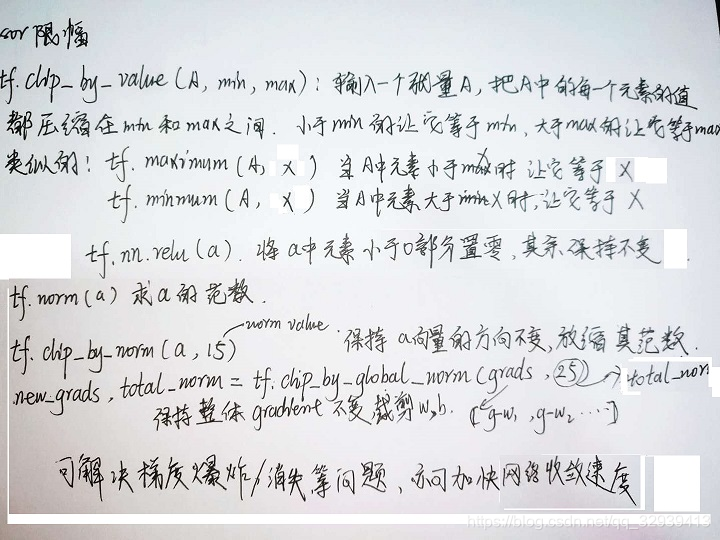
new_grads, total_norm = tf.clip_by_globel_norm(grads, 15) 等比例放缩,不改变数据的分布,不影响梯度方向
3.5.1 clip_by_value
In [149]:a Out[149]:<tf. Tensor: id=422, shape=(10,), dtype=int32, numpy=array([o,1,2,3,
4,5,6,7,8,9], dtype=int32)>
In [150]: tf. maximum(a,2)
0ut[150]:<tf. Tensor: id=426, shape=(10,), dtype=int32, numpy=array([2,2,2,3,
4,5,6,7,8,9], dtype=int32)>
In [151]: tf. minimum(a,8)
Out[151]:<tf. Tensor: id=429, shape=(10,), dtype=int32, numpy=array([o,1,2,3,
4,5,6,7,8,8], dtype=int32)>
In [152]: tf. clip_by_value(a,2,8)
Out[152]:<tf. Tensor: id=434, shape=(10,), dtype=int32, numpy=array([2,2,2,3,
4,5,6,7,8,8], dtype=int32)>
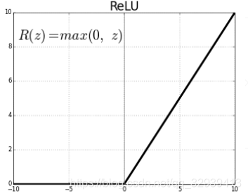
3.5.2 relu
In [153]:a=a-5
Out[154]:<tf. Tensor: id=437, shape=(10,), dtype=int32, numpy=array([-5,-4,-3,
-2,-1,0,1,2,3,4], dtype=int32)>
In [155]: tf. nn. relu(a)
Out[155]:<tf. Tensor: id=439, shape=(10,), dtype=int32, numpy=array([o,0,0,0,
0,0,1,2,3,4], dtype=int32)>
In [156]: tf. maximum(a,0)
Out[156]:<tf. Tensor: id=442, shape=(10,), dtype=int32, numpy=array([o,0,0,0,
0,0,1,2,3,4], dtype=int32)>
3.5.3 clip_by_norm
In [157]:a=tf. random. normal([2,2], mean=10)
<tf. Tensor: id=449, shape=(2,2), dtype=float32, numpy=
array([[12.217459,10.1498375],
[10.84643,10.972536]], dtype=float32)>
In [159]: tf. norm(a)
Out[159]:<tf. Tensor: id=455, shape=(), dtype=float32, numpy=22.14333>
In [161]: aa=tf. clip_by_norm(a,15)
<tf. Tensor: id=473, shape=(2,2), dtype=float32, numpy=
array([[8.276167,6.8755493],
[7.3474245,7.45285]], dtype=float32)>
In [162]: tf. norm(aa)
Out[162]:<tf. Tensor: id=496, shape=(), dtype=float32, numpy=15.000001>
3.5.4 限幅前后对比
print(1==before==1)
for g in grads: print(tf. norm(g))
grads,=tf. clip_by_global_norm(grads,15)
print('==after==1)
for g in grads: print(tf. norm(g))
out:
i@z68:~/TutorialsCN/code_TensorFLow2.0/lesson18-数据限幅$ python main.py
2.0.0-dev20190225
X:(60000,28,28)y:(60000,10)sample:(128,28,28)(128,10)
==before==
tf.Tensor(118.00854,shape=(),dtype=f loat32)
tf.Tensor(3.5821552,shape=(),dtype=float32)tf.Tensor(146.76697,shape=(),dtype=float32)
tf.Tensor(2.830059,shape=(),dtype=float32)
tf.Tensor(183.28879,shape=(),dtype=float32)tf.Tensor(3.4088597,shape=(),dtype=float32)
==after==
tf.Tensor(6.734187,shape=(),dtype=float32)
tf.Tensor(0.20441659,shape=(),dtype=f loat32)
tf.Tensor(8.375294,shape=(),dtype=float32)
tf.Tensor(0.16149803,shape=(),dtype=f loat32)
tf.Tensor(10.45942,shape=(),dtype=float32)
tf.Tensor(0.19452743,shape=(),dtype=f loat32)
0Loss:41.25679016113281
3.6 其它高阶操作
3.6.1 Where
indices=tf.where(a>0) 返回所有为True的坐标,配合tf.gather_nd(a, indices)使用
有两种用法:
1、tf.where(tensor)
tensor 为一个bool 型张量,where函数将返回其中为true的元素的索引。
In [3]:a=tf. random. normal([3,3])
<tf. Tensor: id=11, shape=(3,3), dtype=float32, numpy=
array([[ 1.6420907,0.43938753,-0.31872085],
		[1.144599,-0.02425919,-0.9576591],
		[1.5931814,0.1182256,-0.39948994]], dtype=float32)>
In [5]: mask=a>0
<tf. Tensor: id=14, shape=(3,3), dtype=bool, numpy=
array([[ True, True, False],
		[ True, False, False],
		[ True, True, False]])>
In [7]: tf. boolean_mask(a, mask)
<tf. Tensor: id=42, shape=(5,), dtype=float32, numpy=
array([1.6420907,0.43938753,1.144599,1.5931814,0.1182256], dtype=float32)>
In [8]: indices=tf. where(mask)
<tf. Tensor: id=44, shape=(5,2), dtype=int64, numpy=
array([[0,0],
		[0,1],
		[1,0],
		[2,0],
		[2,1]])>
In [10]: tf. gather_nd(a, indices)
<tf. Tensor: id=46, shape=(5,), dtype=float32, numpy=
array([1.6420907,0.43938753,1.144599,1.5931814,0.1182256], dtype=float32)>
2、tf.where(tensor,a,b)
a,b为和tensor相同维度的tensor,将tensor中的true位置元素替换为a中对应位置元素,false的替换为b中对应位置元素。
In [11]: mask
<tf. Tensor: id=14, shape=(3,3), dtype=bool, numpy=
array([[ True, True, False],
		[ True, False, False],
		[ True, True, False]])>
In [12]:A=tf. ones([3,3])
In [13]:B=tf. zeros([3,3])
In [14]: tf. where(mask,A,B)
<tf. Tensor: id=55, shape=(3,3), dtype=float32, numpy=
array([[1.,1.,0.],
		[1.,0.,0.],
		[1.,1.,0.], dtype=float32)>
3.6.2 tf.scatter_nd
根据indices将updates散布到新的(初始为零)张量。
根据索引对给定shape的零张量中的单个值或切片应用稀疏updates来创建新的张量。此运算符是tf.gather_nd运算符的反函数,它从给定的张量中提取值或切片。
In [17]: indices=tf. constant([[4],[3],[1],[7]])
In[18]: updates=tf. constant([9,10,11,12])
In [19]: shape=tf. constant([8])
In [20]: tf. scatter_nd(indices, updates, shape)
Out[20]:<tf. Tensor: id=60, shape=(8,), dtype=int32, numpy=array([ 0,11,0,10,
9,0,0,12], dtype=int32)>
警告:更新应用的顺序是非确定性的,所以如果indices包含重复项的话,则输出将是不确定的。
3.6.3 tf.meshgrid(x, y)
tf.meshgrid( *args, **kwargs )用于从数组a和b产生网格。生成的网格矩阵A和B大小是相同的。它也可以是更高维的。用法: [A,B]=Meshgrid(a,b),生成size(b) * size(a)大小的矩阵A和B。它相当于a从一行重复增加到size(b)行,把b转置成一列再重复增加到size(a)列
参考W3Cschool:TensorFlow张量变换:tf.meshgrid
四、神经网络与全连接
4.1 数据加载
4.1.1 load_data()和from_tensor_slices()
keras.datasets.xxx.load_data()从网络上加载数据集xxx,格式为numpy数组
(x, y), (x_test, y_test) = keras.datasets.mnist.load_data() # 加载mnist数据集
(x, y), (x_test, y_test) = keras.datasets.cifar10.load_data() # 加载cifar10数据集
tf.data.Dataset.from_tensor_slices在转化数据集时经常会使用这个函数,作用是切分传入的 Tensor 的第一个维度,生成相应的 dataset 。
one_hot 编码,B站小姐姐讲的挺好
Step0: 准备要加载的numpy数据
Step1: 使用 tf.data.Dataset.from_tensor_slices() 函数进行加载
Step2: 使用 shuffle() 打乱数据
Step3: 使用 map() 函数进行预处理
Step4: 使用 batch() 函数设置 batch size 值
Step5: 根据需要 使用 repeat() 设置是否循环迭代数据集
使用tf.data.Dataset.from_tensor_slices五步加载数据集-原文链接
# 版权声明:本程序为引用CSDN博主「rainweic」,并稍作修改
# 原文链接:https://blog.csdn.net/rainweic/article/details/95737315
import tensorflow as tf
from tensorflow import keras

def load_dataset():
	# Step0 准备数据集, 可以是自己动手丰衣足食, 也可以从 tf.keras.datasets 加载需要的数据集(获取到的是numpy数据)
	# 这里以 mnist 为例
	(x, y), (x_test, y_test) = keras.datasets.mnist.load_data()

	# Step1 使用 tf.data.Dataset.from_tensor_slices 进行加载,切分第一个维度
	db_train = tf.data.Dataset.from_tensor_slices((x, y))
	db_test = tf.data.Dataset.from_tensor_slices((x_test, y_test))

	# Step2 打乱数据顺序
	# 从data数据集中按顺序抽取buffer_size个样本放在buffer中,然后打乱buffer中的样本
	# buffer中样本个数不足buffer_size,继续从data数据集中安顺序填充至buffer_size,
	# 此时会再次打乱
	db_train.shuffle(buffer_size=1000)
	db_test.shuffle(buffer_size=1000)

	# Step3 预处理 (预处理函数在下面),这里相当于将db_train、db_test分别进行preprocess函数预处理,并返回自身
	db_train.map(preprocess)
	db_test.map(preprocess)

	# Step4 设置 batch size 一次喂入64个数据
	db_train.batch(64)
	db_test.batch(64)

	# Step5 设置迭代次数(迭代2次) test数据集不需要emmm
	db_train.repeat(2)

	return db_train, db_test

def preprocess(labels, images):
	'''
	最简单的预处理函数:
		转numpy为Tensor、分类问题需要处理label为one_hot编码、处理训练数据
	'''
	# 把numpy数据转为Tensor
	labels = tf.cast(labels, dtype=tf.int32)
	# labels 转为one_hot编码
	labels = tf.one_hot(labels, depth=10)
	# 顺手归一化
	images = tf.cast(images, dtype=tf.float32) / 255
	return labels, images
4.1.2 iter()函数与next()函数
tensorflow2.0之iter()函数与next()函数
1.迭代器是访问集合元素的一种方式。迭代的对象从集合的第一个元素开始访问,直到所有的元素被访问完结束。迭代器只能往前不会后退。
2.next函数:返回迭代器的下一个元素 iter函数:返回迭代器对象本身
3.术语中“可迭代的”指的是支持iter的一个对象(如:iter([1,2,3,4])),而“迭代器”指的是iter所返回的一个支持next(I)的对象。
版权声明:本文为CSDN博主「flyer飞亚」的原创文章
原文链接:https://blog.csdn.net/weixin_43544406/article/details/103091988
#iter()将一个可以迭代的对象转为迭代器对象。
>>>x = [5,6,7,8]
>>> y = iter(x)
>>> y.next()
5
>>> y.next()
6
>>> y.next()
7
db=tf.data.Dataset.from_tensor_slices((x, y)).batch(16).repeat(2) # 相当于数据翻了倍
itr = iter(db)
for i in range(10):
    print(next(itr)[0][15][16,16,0])  # batch中最后一张图中的一个像素
4.2 全连接层
net=tf.keras.layers.Dense(units) dense :全连接层 相当于添加一个层
参数:units:正整数,输出空间的维数。
更多参数参考官网tf.keras.layers.Dense
net.build(input_shape=(None, 784))根据输入shape创建net的所有变量 w ,b,初始化作用
In [3]: net=tf. keras. layers. Dense(10)
In [4]: net. bias
# AttributeError:' Dense' object has no attribute ' bias In [5]: net. get_weights()
0ut[5]:[]
In [6]: net. weights out[6]:[]
In [13]: net. build(input_shape=(None,4)) In [14]: net. kernel. shape, net. bias. shape
0ut[14]:(TensorShape([4,10]), Tensorshape([10]))
In [15]: net. build(input_shape=(None,20))
In [16]: net. kernel. shape, net. bias. shape
0ut[16]:(TensorShape([20,10]), TensorShape([10]))
model.summary()打印网络信息
Sequential模型可以输入由多个训练层组成的列表作为输入参数,并使用add()添加新的训练层。
x = tf.random.normal([2, 3])

model = keras.Sequential([
		keras.layers.Dense(2, activation='relu'),
		keras.layers.Dense(2, activation='relu'),
		keras.layers.Dense(2)
	])
model.build(input_shape=[None, 3])
model.summary()

for p in model.trainable_variables:
	print(p.name, p.shape)
out:
Model: "sequential"
_________________________________________________________________
Layer (type)                 Output Shape              Param #
=================================================================
dense (Dense)                multiple                  8
_________________________________________________________________
dense_1 (Dense)              multiple                  6
_________________________________________________________________
dense_2 (Dense)              multiple                  6
=================================================================
Total params: 20
Trainable params: 20
Non-trainable params: 0
_________________________________________________________________
dense/kernel:0 (3, 2)
dense/bias:0 (2,)
dense_1/kernel:0 (2, 2)
dense_1/bias:0 (2,)
dense_2/kernel:0 (2, 2)
dense_2/bias:0 (2,)
4.3 输出方式
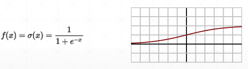
4.3.1 sigmoid
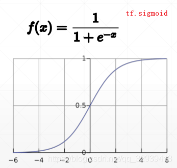
tf.sigmoid 将一个输出映射到(0,1)的区间
In [21]:a=tf. linspace(-2.,2,5)
In [22]: tf. sigmoid(a)
<tf. Tensor: id=54, shape=(5,), dtype=float32, numpy=
array([o.11920291,0.26894143,0.5,0.7310586,0.880797], dtype=f loat32)>
4.3.2 Softmax
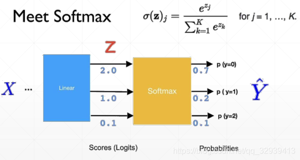
prob=tf.nn.softmax(logits)保证所有输出之和=1, logits一般指没有激活函数的最后一层的输出
In [23]: tf. nn. softmax(a)
<tf. Tensor: id=56, shape=(5,), dtype=float32, numpy=
array([0.01165623,0.03168492,0.08612854,0.23412167,0.6364086], dtype=float32)>
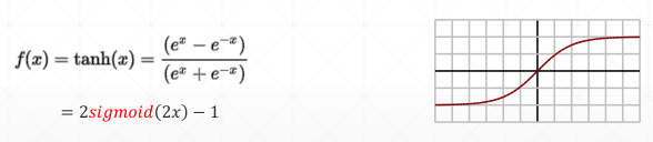
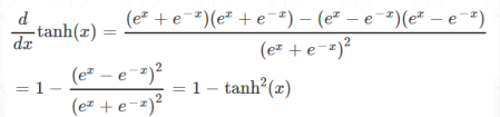
4.3.3 tanh
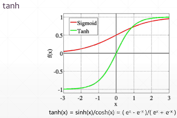
tf.tanh将一个输出映射到输出在 [-1, 1]之间
In [30]:a Out[30]:<tf. Tensor: id=53, shape=(5,), dtype=float32, numpy=array([-2.,-1.,0.,
1.,2.], dtype=float32)>
In [33]: tf. tanh(a)
<tf. Tensor: id=73, shape=(5,), dtype=float32, numpy=
array([-8.9640276,-0.7615942,8.,0.7615942,0.9640276], dtype=f loat32)>
函数分类大PK:Sigmoid和Softmax,分别怎么用?
4.4 误差计算
4.4.1 MSE(均方误差)
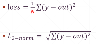
tf.reduce_mean(tf.losses.MSE(y, out))
import tensorflow as tf
y = tf.constant([1, 2, 3, 0, 2])
y = tf.one_hot(y, depth=4)
y = tf.cast(y, dtype=tf.float32)
out = tf.random.normal([5, 4])

loss1 = tf.reduce_mean(tf.square(y-out))
loss2 = tf.square(tf.norm(y-out))/(5*4)
loss3 = tf.reduce_mean(tf.losses.MSE(y, out)) # VS MeanSquaredError is a class

print(loss1)
print(loss2)
print(loss3)
Out(三种效果差不多):
tf.Tensor(1.4607859, shape=(), dtype=float32)
tf.Tensor(1.4607859, shape=(), dtype=float32)
tf.Tensor(1.4607859, shape=(), dtype=float32)
4.4.2 交叉熵 -log(q_i)
辅助理解:一文搞懂交叉熵在机器学习中的使用,透彻理解交叉熵背后的直觉
tf.losses.categorical_crossentropy的效果:
In [15]: tf. losses. categorical_crossentropy([0,1,0,0],[0.25,0.25,0.25,0.25])
Out[15]:<tf. Tensor: id=98, shape=(), dtype=float32, numpy=1.3862944>
In [16]: tf. losses. categorical_crossentropy([0,1,0,0],[0.1,0.1,0.8,0.1])
Out[16]:<tf. Tensor: id=117, shape=(), dtype=float32, numpy=2.3978953>
In [17]: tf. losses. categorical_crossentropy([0,1,0,0],[0.1,0.7,0.1,0.1])
Out[17]:<tf. Tensor: id=136, shape=(), dtype=float32, numpy=0.35667497>
In [18]: tf. losses. categorical_crossentropy([0,1,0,0],[0.01,0.97,0.01,0.01])
Out[18]:<tf. Tensor: id=155, shape=(), dtype=float32, numpy=0.030459179>
tf.losses.categorical_crossentropy(y, logits, from_logits=True)其中,使用from_logits=True参数相当于自动添加softmax,从而不用手动添加softmax,而且在大多数情况下这样使用可以避免数据不稳定问题
In [24]:x=tf. random. normal([1,784]) In [25]:w=tf. random. normal([784,2])
In [26]:b=tf. zeros([2])
In [27]: Logits=x@w+b Out[29]:<tf. Tensor: id=299, shape=(1,2), dtype=float32, numpy=array([[-26.27812,
28.63038]], dtype=float32)>
In [30]: prob=tf. math. softmax(logits, axis=1)
0ut[31]:<tf. Tensor: id=301, shape=(1,2), dtype=f loat32, numpy=array([[1.4241021e-24,1.0000000e+00]], dtype=float32)>
In [34]: tf. losses. categorical_crossentropy([0,1], logits, from_logit s=True)
Out[34]:<tf. Tensor: id=393, shape=(1,), dtype=float32, numpy=array([0.], dtype=f loat32)>
In [35]: tf. losses. categorical_crossentropy([0,1], prob)
Out[35]:<tf. Tensor: id=411, shape=(1,), dtype=float32, numpy=array([1.192093e-
07], dtype=float32)>
tf.losses.binary_crossentropy(x, y) 常用于计算二分类问题
In [20]: criteon([o,1,0,0],[0.1,0.7,0.1,0.1])
Out[20]:<tf. Tensor: id=186, shape=(), dtype=float32, numpy=0.35667497>
In[21]: criteon([o,1],[0.9,0.1])
0ut[21]:<tf. Tensor: id=216, shape=(), dtype=float32, numpy=2.3025851>
In [22]: tf. losses. BinaryCrossentropy()([1],[0.1])
Out[22]:<tf. Tensor: id=254, shape=(), dtype=float32, numpy=2.3025842>
In [23]: tf. losses. binary_crossentropy([1],[0.1])
0ut[23]:<tf. Tensor: id=281, shape=(), dtype=float32, numpy=2.3025842>
五、梯度计算
导数 => 偏微分 某个坐标方向的导数=>梯度所有坐标方向导数的集合
5.1 自动求梯度
with tf.GradientTape(persistent=True) as tape: 其中persistent=True可暂时保持内存中的数据不释放,使得tape.gradient可被多次调用
with tf.GradientTape() as tape:
    loss= ...
    [w_grad] = tape.gradiet(loss, [w])  # w是指定要求梯度的参数
    [w_grad] = tape.gradient(loss, model.trainable_variables) # model是链接关系,trainable_variables表示链接中所有可训练参数,即可自动得到训练参数

**求二阶导:**

```python
with tf.GradientTape() as t1:
    with tf.GradientTape() as t2:
        y = x * w + b
    dy_dw, dy_db = t2.gradient(y, [w, b])

d2y_dw2 = t1.gradient(dy_dw, w)
5.2 激活函数及其梯度
5.2.1 sigmoid
sigmoid梯度:
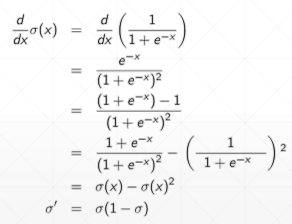
a=tf. linspace(-10.,10.,10)
with tf. GradientTape() as tape:
tape. watch(a)
y=tf. sigmoid(a)
grads=tape. gradient(y,[a])
x:[-10.-7.7777777-5.5555553-3.333333-1.1111107 1.11111163.3333345.55555637.777778610.]
y:[4.5388937e-054.1878223e-04 3.8510561e-033.4445226e-02 2.4766389e-017.5233626e-01 9.6555483e-01 9.9614894e-019.9958128e-01 9.9995458e-01]
grad:[4.5386874e-05 4.1860685e-043.8362255e-033.3258751e-02 1.8632649e-011.8632641e-013.3258699e-023.8362255e-034.1854731e-044.5416677e-05]
其中tape. watch(a),的一点说明:自动trace可训练参数(不用watch),Tensors可以在上下文管理器中调用watch()方法来trace(需要watch)。
5.2.2 tanh
tanh梯度:
In [5]:a=tf. linspace(-5.,5.,10)
In [6]: tf. tanh(a)
0ut[6]:
<tf. Tensor: id=10, shape=(10,), dtype=float32, numpy=
array([-0.9999092,-0.9991625,-0.99229795,-0.9311096,-0.50467217,
0.5046725,0.93110967,0.99229795,0.9991625,0.9999092]
dtype=float32)>
5.2.3 relu
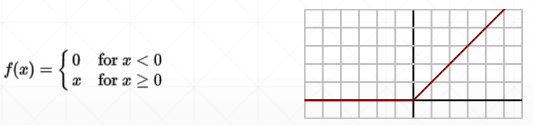
relu梯度:
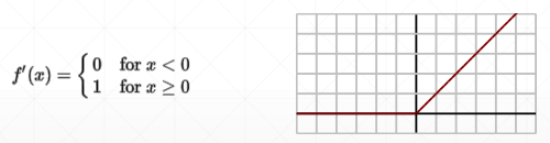
In [11]:a=tf. linspace(-1.,1.,10)
In [12]: tf. nn. relu(a
<tf. Tensor: id=24, shape=(10,), dtype=float32, numpy=
array([0.,0.,0.,0.,0.
0.11111116,0.33333337,0.5555556,0.7777778,1.], dtype=float32)>
In [13]: tf. nn. leaky_relu(a)
<tf. Tensor: id=26, shape=(10,), dtype=float32, numpy=
array([-0.2,-0.15555556,-0.11111112,-0.06666666,-0.02222222,
0.11111116,0.33333337,0.5555556,0.7777778,1.], dtype=float32)>
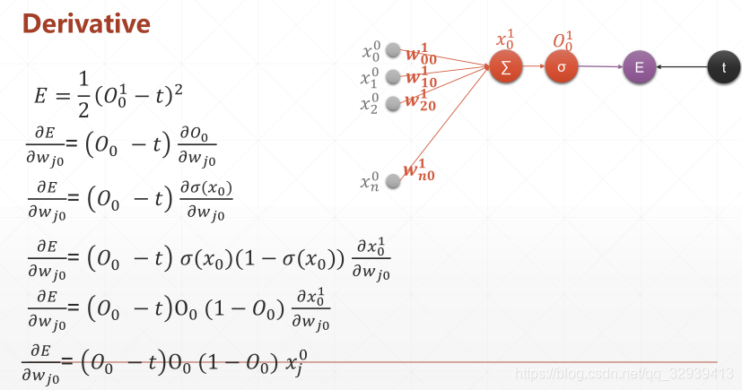
5.3 反向传播
5.3.1 单层输出感知机
x=tf. random. normal([1,3])
w=tf. ones([3,1])
b=tf. ones([1])
y=tf. constant([1])
with tf. GradientTape() as tape: tape. watch([w,b])
logits=tf. sigmoid(xQw+b)
loss=tf. reduce_mean(tf. losses. MSE(y, logits))
grads=tape. gradient(loss,[w,b])
w grad: tf. Tensor(
[[-0.00478814]
[-0.00588211]
[0.00186196]], shape=(3,1), dtype=float32)
b grad: tf. Tensor([-0.00444918], shape=(1,), dtype=float32)
5.3.2 多层输出感知机
In [3]:x=tf. random. normal([2,4]) In [4]:w=tf. random. normal([4,3])
In [5]:b=tf. zeros([3])
In [6]:y=tf. constant([2,0])
In [9]: with tf. GradientTape() as tape: tape. watch([w,b])
prob=tf. nn. softmax(x@w+b, axis=1)
loss=tf. reduce_mean(tf. losses. MSE(tf. one_hot(y, depth=3), prob))
In [10]: grads=tape. gradient(1oss,[w,b])
In [11]: grads[0]
[[-0.00967887,-0.00335512,0.01303399],
[-0.04446869,0.06194263,-0.01747394],
[-0.04530644,0.01043231,0.03487412],
[0.02006017,-0.03638988,0.0163297]]
In [12]: grads[1]#[-0.02585024,0.06217915,-0.03632889]
5.3.3 链式法则
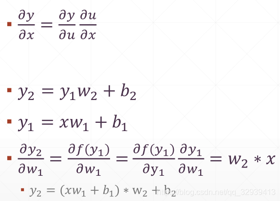
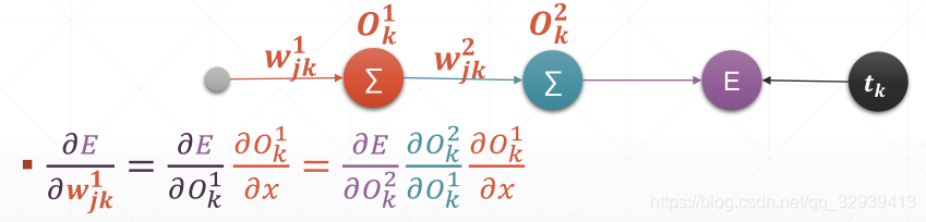
x=tf. constant(1.)
w1=tf. constant(2.)
b1=tf. constant(1.)
w2=tf. constant(2.)
b2=tf. constant(1.)
with tf. GradientTape(persistent=True) as tape:
tape. watch([w1,b1,w2,b2])
y1=x*W1+b1
y2=y1*W2+b2
dy2_dy1=tape. gradient(y2,[y1])[0]
dy1_dw1=tape. gradient(y1,[w1])[0]
dy2_dw1=tape. gradient(y2,[w1])[0]
tf. Tensor(2.0, shape=(), dtype=float32)
tf. Tensor(2.0, shape=(), dtype=float32)
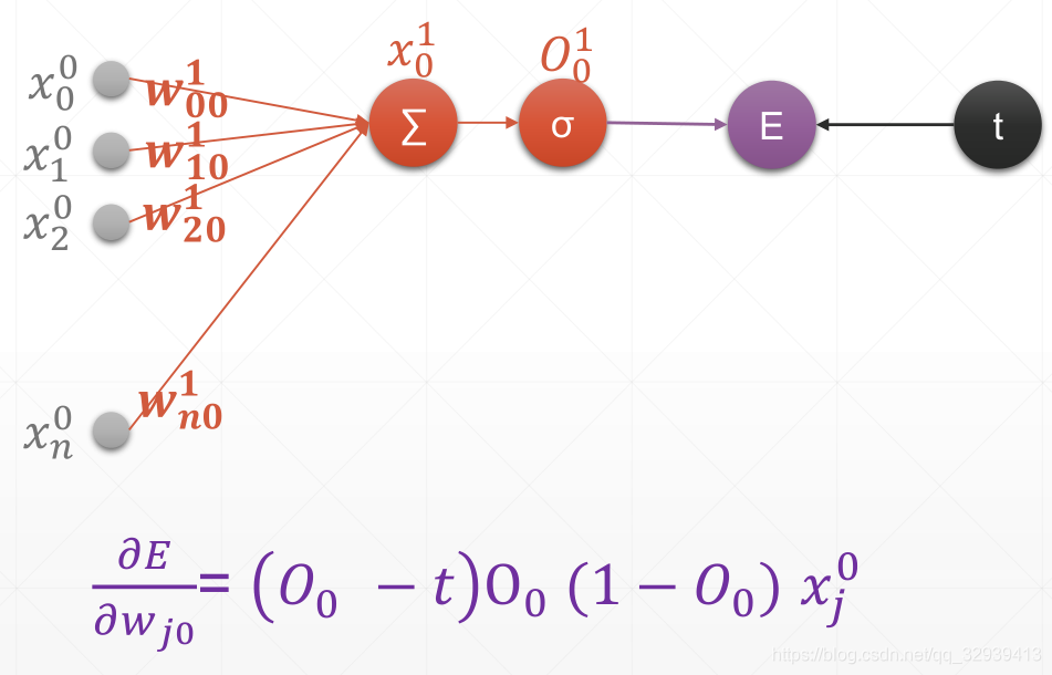
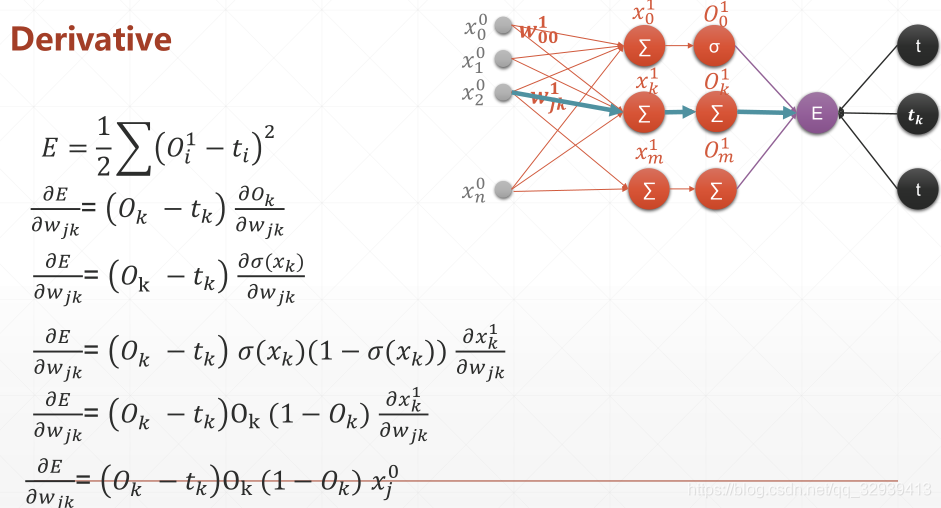
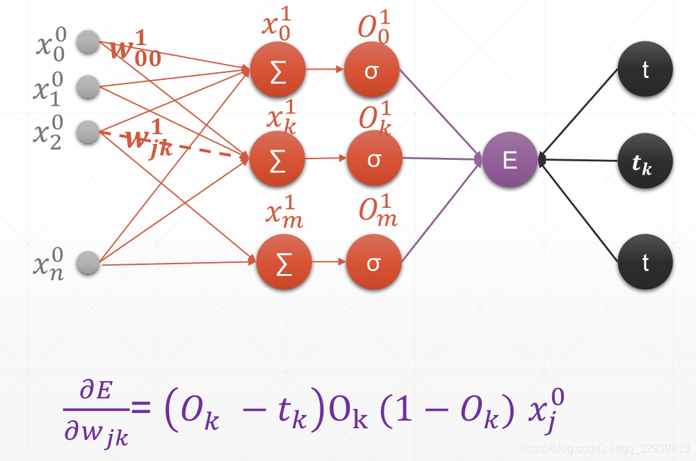
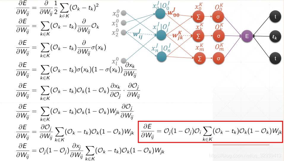
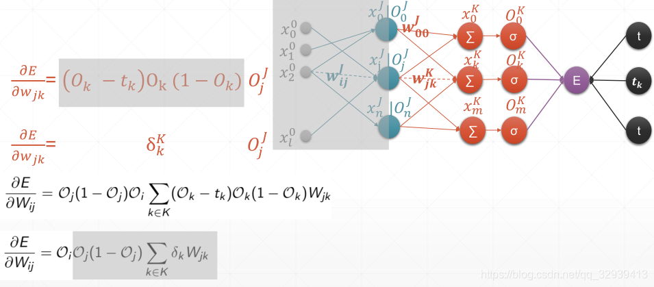
5.3.4 多层感知机梯度
5.4 损失函数优化实战
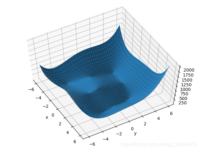
假设损失函数:
import numpy as np
from mpl_toolkits.mplot3d import Axes3D
from matplotlib import pyplot as plt
import tensorflow as tf


def himmelblau(x):
    return (x[0] ** 2 + x[1] - 11) ** 2 + (x[0] + x[1] ** 2 - 7) ** 2

# -------------绘图-----------------
x = np.arange(-6, 6, 0.1)
y = np.arange(-6, 6, 0.1)
print('x,y range:', x.shape, y.shape)
X, Y = np.meshgrid(x, y)
print('X,Y maps:', X.shape, Y.shape)
Z = himmelblau([X, Y])

fig = plt.figure('himmelblau')
ax = fig.gca(projection='3d')
ax.plot_surface(X, Y, Z)
ax.view_init(60, -30)
ax.set_xlabel('x')
ax.set_ylabel('y')
plt.show()
# ------------绘图-------------------
# [1., 0.], [-4, 0.], [4, 0.]
x = tf.constant([-4., 0.])

for step in range(200):

    with tf.GradientTape() as tape:
        tape.watch([x])
        y = himmelblau(x)

    grads = tape.gradient(y, [x])[0]
    x -= 0.01 * grads

    if step % 20 == 0:
        print('step {}: x = {}, f(x) = {}'
              .format(step, x.numpy(), y.numpy()))
Out:
step 0: x = [-2.98       -0.09999999], f(x) = 146.0
step 20: x = [-3.6890156 -3.1276684], f(x) = 6.054738998413086
step 40: x = [-3.7793102 -3.283186 ], f(x) = 0.0
step 60: x = [-3.7793102 -3.283186 ], f(x) = 0.0
step 80: x = [-3.7793102 -3.283186 ], f(x) = 0.0
step 100: x = [-3.7793102 -3.283186 ], f(x) = 0.0
step 120: x = [-3.7793102 -3.283186 ], f(x) = 0.0
step 140: x = [-3.7793102 -3.283186 ], f(x) = 0.0
step 160: x = [-3.7793102 -3.283186 ], f(x) = 0.0
step 180: x = [-3.7793102 -3.283186 ], f(x) = 0.0
之后就可以通过层的方式完成实战了!!!
5.5 手写数字问题实战(层)
import os

os.environ['TF_CPP_MIN_LOG_LEVEL'] = '2'

import tensorflow as tf
from tensorflow import keras
from tensorflow.keras import datasets, layers, optimizers, Sequential, metrics


def preprocess(x, y):
    x = tf.cast(x, dtype=tf.float32) / 255.
    y = tf.cast(y, dtype=tf.int32)
    return x, y


(x, y), (x_test, y_test) = datasets.fashion_mnist.load_data()
print(x.shape, y.shape)
db_train = tf.data.Dataset.from_tensor_slices((x, y))
db_test = tf.data.Dataset.from_tensor_slices((x_test, y_test))
db_train = db_train.map(preprocess).shuffle(buffer_size=10000).batch(batch_size=128)
db_test = db_test.map(preprocess).shuffle(buffer_size=10000).batch(batch_size=128)

# db_iter = iter(db_train)
# sample = next(db_iter)
# print("batch:", sample[0].shape, sample[1].shape)

model = Sequential([
    layers.Dense(256, activation=tf.nn.relu),  # [b, 784] => [b, 256]
    layers.Dense(128, activation=tf.nn.relu),  # [b, 256] => [b, 128]
    layers.Dense(64, activation=tf.nn.relu),  # [b, 128] => [b, 64]
    layers.Dense(32, activation=tf.nn.relu),  # [b, 64] => [b, 32]
    layers.Dense(10)  # [b, 32] => [b, 10], 330 = 32*10 + 10
])
model.build(input_shape=[None, 28 * 28])
model.summary()
# w = w - lr*grad
optimizer = optimizers.Adam(lr=1e-3)


def main():
    for epoch in range(30):

        for step, (x, y) in enumerate(db_train):
            # x: [b, 28, 28] => [b, 784]
            # y: [b]
            x = tf.reshape(x, [-1, 28 * 28])

            with tf.GradientTape() as tape:
                # [b, 784] => [b, 10]
                logits = model(x)
                y_onehot = tf.one_hot(y, depth=10)
                loss_mse = tf.reduce_mean(tf.losses.MSE(y_onehot, logits))
                loss_ce = tf.reduce_mean(tf.losses.categorical_crossentropy(y_onehot, logits, from_logits=True))
            grads = tape.gradient(loss_ce, model.trainable_variables)
            optimizer.apply_gradients(zip(grads, model.trainable_variables))
            if step % 100 == 0:
                print(epoch, step, 'loss:', float(loss_ce), float(loss_mse))
        # test
        total_correct = 0
        total_num = 0

        for x, y in db_test:
            # x: [b, 28, 28] => [b, 784]
            # y: [b]
            x = tf.reshape(x, [-1, 28 * 28])
            # [b, 10]
            logits = model(x)
            # logits => prob, [b, 10]
            prob = tf.nn.softmax(logits, axis=1)
            # [b, 10] => [b], int64
            pred = tf.argmax(prob, axis=1)
            pred = tf.cast(pred, dtype=tf.int32)
            # pred:[b]
            # y: [b]
            # correct: [b], True: equal, False: not equal
            correct = tf.equal(pred, y)
            correct = tf.reduce_sum(tf.cast(correct, dtype=tf.int32))

            total_correct += int(correct)
            total_num += x.shape[0]

        acc = total_correct / total_num
        print(epoch, 'test acc:', acc)


if __name__ == '__main__':
    main()
OUT:
(60000, 28, 28) (60000,)
Model: "sequential"
_________________________________________________________________
Layer (type)                 Output Shape              Param #
=================================================================
dense (Dense)                multiple                  200960
_________________________________________________________________
dense_1 (Dense)              multiple                  32896
_________________________________________________________________
dense_2 (Dense)              multiple                  8256
_________________________________________________________________
dense_3 (Dense)              multiple                  2080
_________________________________________________________________
dense_4 (Dense)              multiple                  330
=================================================================
Total params: 244,522
Trainable params: 244,522
Non-trainable params: 0
_________________________________________________________________
0 0 loss: 2.3679399490356445 0.19908082485198975
0 100 loss: 0.6205164194107056 21.134510040283203
0 200 loss: 0.5330268144607544 20.619508743286133
0 300 loss: 0.4956797659397125 23.731096267700195
0 400 loss: 0.4412800371646881 22.34198760986328
0 test acc: 0.8525
1 0 loss: 0.33451998233795166 21.35747718811035
1 100 loss: 0.41022008657455444 22.784833908081055
1 200 loss: 0.24400854110717773 21.5227108001709
1 300 loss: 0.3893822431564331 23.128589630126953
1 400 loss: 0.3844433128833771 22.818313598632812
1 test acc: 0.8603

......

28 0 loss: 0.06723682582378387 178.3081512451172
28 100 loss: 0.11262191832065582 196.36248779296875
28 200 loss: 0.1300932615995407 196.3513641357422
28 300 loss: 0.11398142576217651 189.61363220214844
28 400 loss: 0.12036384642124176 201.0360107421875
28 test acc: 0.8909
29 0 loss: 0.13888132572174072 175.87173461914062
29 100 loss: 0.09474453330039978 169.97776794433594
29 200 loss: 0.10801658034324646 194.08380126953125
29 300 loss: 0.1834179162979126 263.3036804199219
29 400 loss: 0.09733995050191879 251.29617309570312
29 test acc: 0.8898
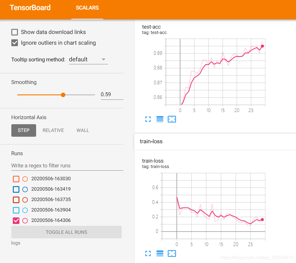
六、 Tensorboard可视化
6.1 数据可视化
tensorboard --logdir logs
Step1:创建日志写入地址,文件夹名为logs
current_time = datetime.datetime.now().strftime("%Y%m%d-%H%M%S")
log_dir = 'logs/' + current_time
summary_writer = tf.summary.create_file_writer(log_dir)
Step2:喂入监听数据,设置时间戳
        with summary_writer.as_default():
            tf.summary.scalar('train-loss', float(loss_ce), step=epoch) #此处时间戳为epoch
            tf.summary.scalar('test-acc', float(acc), step=epoch)
Step3:打开监听
使用Terminal进入程序文件根目录,输入tensorboard --logdir logs其中logs对应第一步中文件夹名
(base) PS X:\PythonWorkStation\TF> tensorboard --logdir logs
2020-05-06 16:30:31.548573: I tensorflow/stream_executor/platform/default/dso_loader.cc:44] Successfully opened dynamic library cudart64_101.dll
Serving TensorBoard on localhost; to expose to the network, use a proxy or pass --bind_all
TensorBoard 2.1.1 at http://localhost:6006/ (Press CTRL+C to quit)
Step4:打开WEB端
浏览器汇总打开上一步中的http://localhost:6006/
Code:
import os

os.environ['TF_CPP_MIN_LOG_LEVEL'] = '2'
import datetime
import tensorflow as tf
from tensorflow import keras
from tensorflow.keras import datasets, layers, optimizers, Sequential, metrics


def preprocess(x, y):
    x = tf.cast(x, dtype=tf.float32) / 255.
    y = tf.cast(y, dtype=tf.int32)
    return x, y


(x, y), (x_test, y_test) = datasets.fashion_mnist.load_data()
print(x.shape, y.shape)
db_train = tf.data.Dataset.from_tensor_slices((x, y))
db_test = tf.data.Dataset.from_tensor_slices((x_test, y_test))
db_train = db_train.map(preprocess).shuffle(buffer_size=10000).batch(batch_size=128)
db_test = db_test.map(preprocess).shuffle(buffer_size=10000).batch(batch_size=128)

# db_iter = iter(db_train)
# sample = next(db_iter)
# print("batch:", sample[0].shape, sample[1].shape)

model = Sequential([
    layers.Dense(256, activation=tf.nn.relu),  # [b, 784] => [b, 256]
    layers.Dense(128, activation=tf.nn.relu),  # [b, 256] => [b, 128]
    layers.Dense(64, activation=tf.nn.relu),  # [b, 128] => [b, 64]
    layers.Dense(32, activation=tf.nn.relu),  # [b, 64] => [b, 32]
    layers.Dense(10)  # [b, 32] => [b, 10], 330 = 32*10 + 10
])
model.build(input_shape=[None, 28 * 28])
model.summary()
# w = w - lr*grad
optimizer = optimizers.Adam(lr=1e-3)

# tensorboard可视化 Step1 build summary------------------------------
current_time = datetime.datetime.now().strftime("%Y%m%d-%H%M%S")
log_dir = 'logs/' + current_time
summary_writer = tf.summary.create_file_writer(log_dir)
# tensorboard可视化 Step1 build summary------------------------------

def main():
    for epoch in range(30):

        for step, (x, y) in enumerate(db_train):
            # x: [b, 28, 28] => [b, 784]
            # y: [b]
            x = tf.reshape(x, [-1, 28 * 28])

            with tf.GradientTape() as tape:
                # [b, 784] => [b, 10]
                logits = model(x)
                y_onehot = tf.one_hot(y, depth=10)
                loss_mse = tf.reduce_mean(tf.losses.MSE(y_onehot, logits))
                loss_ce = tf.reduce_mean(tf.losses.categorical_crossentropy(y_onehot, logits, from_logits=True))
            grads = tape.gradient(loss_ce, model.trainable_variables)
            optimizer.apply_gradients(zip(grads, model.trainable_variables))
            if step % 100 == 0:
                print(epoch, step, 'loss:', float(loss_ce), float(loss_mse))

                # test
        total_correct = 0
        total_num = 0

        for x, y in db_test:
            # x: [b, 28, 28] => [b, 784]
            # y: [b]
            x = tf.reshape(x, [-1, 28 * 28])
            # [b, 10]
            logits = model(x)
            # logits => prob, [b, 10]
            prob = tf.nn.softmax(logits, axis=1)
            # [b, 10] => [b], int64
            pred = tf.argmax(prob, axis=1)
            pred = tf.cast(pred, dtype=tf.int32)
            # pred:[b]
            # y: [b]
            # correct: [b], True: equal, False: not equal
            correct = tf.equal(pred, y)
            correct = tf.reduce_sum(tf.cast(correct, dtype=tf.int32))

            total_correct += int(correct)
            total_num += x.shape[0]

        acc = total_correct / total_num
        print(epoch, 'test acc:', acc)

        # tensorboard可视化 Step2 fed scalar------------------------------
        with summary_writer.as_default():
            tf.summary.scalar('train-loss', float(loss_ce), step=epoch)
            tf.summary.scalar('test-acc', float(acc), step=epoch)
		# tensorboard可视化 Step2 fed scalar------------------------------

if __name__ == '__main__':
    main()
6.2 图片可视化
1.单张图
# get xfrom(x,y)
sample_img=next(iter(db))[0]
# get first image instance sample_img=sample_img[0]
sample_img=tf. reshape(sample_img,[1,28,28,1])
with summary_writer. as_default():
	tf. summary. image("Training sample:", sample_img, step=0)

2.多张图
val_images=x[:25]
val_images=tf. reshape(val_images,[-1,28,28,1])
with summary_writer. as_default():
	tf. summary. image("val-onebyone-images:", val_images, max_outputs=25, step=step)

3.优化显示的多张图
val_images=tf. reshape(val_images,[-1,28,28])
figure =image_grid(val_images)
tf. summary. image("val-images:', plot_to_image(figure), step=step)
其中调用的方法:
from    matplotlib import pyplot as plt

def plot_to_image(figure):
  """Converts the matplotlib plot specified by 'figure' to a PNG image and
  returns it. The supplied figure is closed and inaccessible after this call."""
  # Save the plot to a PNG in memory.
  buf = io.BytesIO()
  plt.savefig(buf, format='png')
  # Closing the figure prevents it from being displayed directly inside
  # the notebook.
  plt.close(figure)
  buf.seek(0)
  # Convert PNG buffer to TF image
  image = tf.image.decode_png(buf.getvalue(), channels=4)
  # Add the batch dimension
  image = tf.expand_dims(image, 0)
  return image

def image_grid(images):
  """Return a 5x5 grid of the MNIST images as a matplotlib figure."""
  # Create a figure to contain the plot.
  figure = plt.figure(figsize=(10,10))
  for i in range(25):
    # Start next subplot.
    plt.subplot(5, 5, i + 1, title='name')
    plt.xticks([])
    plt.yticks([])
    plt.grid(False)
    plt.imshow(images[i], cmap=plt.cm.binary)

七、Keras高层接口
7.1 Metrics
参考:Keras高层API之Metrics
评估函数用于评估当前训练模型的性能。当模型编译后,评价函数应该作为metrics的参数输入;
通俗一点的解释:例如获得loss的均值,之前都是所有的loss全部求解出之后才求均值,但是在训练的过程中有一种需求是实时得到loss的均值,那就需要每产生一个新的loss就喂入,结合之前的所有loss求得实时均值。而可以实现在每个时间戳都能产生实时评估的接口就是Metrics
step1:Build a meter
acc_meter = metrics.Accuracy()
loss_meter = metrics.Mean()
step2:Update data
loss_meter.update_state(loss) # 喂入数据
acc_meter.update_state(y,pred)
step3:Get Average data
print(step,'loss:',loss_meter.result().numpy()) # 产生评估值
print(step,'Evaluate Acc:',total_correct/total,acc_meter.result().numpy())
清除缓存
if step % 100 == 0:
    print(step,'loss:',loss_meter.result().numpy())
    loss_meter.reset_states() # 清除之前的缓冲重新评估

if step % 500 ==0:
    total,total_correct = 0.,0
    acc_meter.reset_states()
实战:
import  tensorflow as tf
from    tensorflow.keras import datasets, layers, optimizers, Sequential, metrics


def preprocess(x, y):

    x = tf.cast(x, dtype=tf.float32) / 255.
    y = tf.cast(y, dtype=tf.int32)

    return x,y


batchsz = 128
(x, y), (x_val, y_val) = datasets.mnist.load_data()
print('datasets:', x.shape, y.shape, x.min(), x.max())


db = tf.data.Dataset.from_tensor_slices((x,y))
db = db.map(preprocess).shuffle(60000).batch(batchsz).repeat(10)

ds_val = tf.data.Dataset.from_tensor_slices((x_val, y_val))
ds_val = ds_val.map(preprocess).batch(batchsz)


network = Sequential([layers.Dense(256, activation='relu'),
                     layers.Dense(128, activation='relu'),
                     layers.Dense(64, activation='relu'),
                     layers.Dense(32, activation='relu'),
                     layers.Dense(10)])
network.build(input_shape=(None, 28*28))
network.summary()

optimizer = optimizers.Adam(lr=0.01)

acc_meter = metrics.Accuracy()
loss_meter = metrics.Mean()


for step, (x,y) in enumerate(db):

    with tf.GradientTape() as tape:
        # [b, 28, 28] => [b, 784]
        x = tf.reshape(x, (-1, 28*28))
        # [b, 784] => [b, 10]
        out = network(x)
        # [b] => [b, 10]
        y_onehot = tf.one_hot(y, depth=10)
        # [b]
        loss = tf.reduce_mean(tf.losses.categorical_crossentropy(y_onehot, out, from_logits=True))

        loss_meter.update_state(loss)


    grads = tape.gradient(loss, network.trainable_variables)
    optimizer.apply_gradients(zip(grads, network.trainable_variables))


    if step % 100 == 0:

        print(step, 'loss:', loss_meter.result().numpy())
        loss_meter.reset_states()


    # evaluate
    if step % 500 == 0:
        total, total_correct = 0., 0
        acc_meter.reset_states()

        for step, (x, y) in enumerate(ds_val):
            # [b, 28, 28] => [b, 784]
            x = tf.reshape(x, (-1, 28*28))
            # [b, 784] => [b, 10]
            out = network(x)


            # [b, 10] => [b]
            pred = tf.argmax(out, axis=1)
            pred = tf.cast(pred, dtype=tf.int32)
            # bool type
            correct = tf.equal(pred, y)
            # bool tensor => int tensor => numpy
            total_correct += tf.reduce_sum(tf.cast(correct, dtype=tf.int32)).numpy()
            total += x.shape[0]

            acc_meter.update_state(y, pred)


        print(step, 'Evaluate Acc:', total_correct/total, acc_meter.result().numpy())
OUT:
Model: "sequential"
_________________________________________________________________
Layer (type)                 Output Shape              Param #
=================================================================
dense (Dense)                multiple                  200960
_________________________________________________________________
dense_1 (Dense)              multiple                  32896
_________________________________________________________________
dense_2 (Dense)              multiple                  8256
_________________________________________________________________
dense_3 (Dense)              multiple                  2080
_________________________________________________________________
dense_4 (Dense)              multiple                  330
=================================================================
Total params: 244,522
Trainable params: 244,522
Non-trainable params: 0
_________________________________________________________________
2020-05-07 20:38:46.837981: I tensorflow/stream_executor/platform/default/dso_loader.cc:44] Successfully opened dynamic library cublas64_10.dll
0 loss: 2.3376217
78 Evaluate Acc: 0.1247 0.1247
100 loss: 0.5312836
200 loss: 0.24513794
300 loss: 0.21127209
400 loss: 0.1908613
500 loss: 0.15478776
......
78 Evaluate Acc: 0.9753 0.9753
4100 loss: 0.065056
4200 loss: 0.07652673
4300 loss: 0.07414787
4400 loss: 0.077764966
4500 loss: 0.07281441
78 Evaluate Acc: 0.9708 0.9708
4600 loss: 0.055623364
7.2 Compile & Fit
对下图内容的封装 ,keras就有了使用compile对其进行封装,使用fit进行迭代epoch训练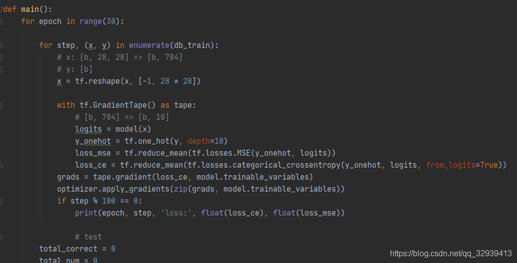
详细参考:tensorflow2的compile & fit函数
7.2.1 compile 配置用于训练的模型
network = Sequential([layers.Dense(256, activation='relu'),
                      layers.Dense(128, activation='relu'),
                      layers.Dense(64, activation='relu'),
                      layers.Dense(32, activation='relu'),
                      layers.Dense(10)])
network.build(input_shape=(None, 28 * 28))
network.summary()
print("--------------------Step1-----------------------")
network.compile(optimizer=optimizers.Adam(lr=0.01),
                loss=tf.losses.CategoricalCrossentropy(from_logits=True),
                metrics=['accuracy']
                )
其中
- optimizer 用来配置模型的优化器
- loss - 用来配置模型的损失函数
- metrics - 用来配置模型评价的方法,如accuracy、mse等,例如实战中:
loss: 2.3259 - accuracy: 0.1094
7.2.2 fit 喂入训练数据
print("--------------------Step2-----------------------")
network.fit(db_train, epochs=5, validation_data=ds_val, validation_freq=2)
此处:
db_train 为训练数据集
epochs 训练批次
validation_data 为测试数据集
validation_freq 意味着每2个epoch做一次验证 例如实战中:- val_loss: 0.1482 - val_accuracy: 0.9604
7.2.3 evaluate返回测试模式下模型的损失值和指标值
print("--------------------Step3-----------------------")
network.evaluate(ds_val)
此处ds_val为喂入的测试集数据,对应实战中:
--------------------Step3-----------------------
 1/79 [..............................] - ETA: 0s - loss: 0.0255 - accuracy: 0.9922
10/79 [==>...........................] - ETA: 0s - loss: 0.1624 - accuracy: 0.9664
19/79 [======>.......................] - ETA: 0s - loss: 0.1717 - accuracy: 0.9589
28/79 [=========>....................] - ETA: 0s - loss: 0.1599 - accuracy: 0.9623
37/79 [=============>................] - ETA: 0s - loss: 0.1601 - accuracy: 0.9620
47/79 [================>.............] - ETA: 0s - loss: 0.1473 - accuracy: 0.9643
57/79 [====================>.........] - ETA: 0s - loss: 0.1345 - accuracy: 0.9679
66/79 [========================>.....] - ETA: 0s - loss: 0.1239 - accuracy: 0.9704
74/79 [===========================>..] - ETA: 0s - loss: 0.1142 - accuracy: 0.9723
7.2.4 predict生成输入样本的输出预测
print("--------------------Step4-----------------------")
sample = next(iter(ds_val))
x = sample[0]
y = sample[1]  # one-hot
pred = network.predict(x)  # [b, 10]
# convert back to number
y = tf.argmax(y, axis=1)
pred = tf.argmax(pred, axis=1)

print(pred)
print(y)
此处输出对应实战中:
--------------------Step4-----------------------
tf.Tensor(
[7 2 1 0 4 1 4 9 5 9 0 6 9 0 1 5 9 7 3 4 9 6 6 5 4 0 7 4 0 1 3 1 3 4 7 2 7
 1 2 1 1 7 4 2 3 5 1 2 4 4 6 3 5 5 6 0 4 1 9 5 7 8 9 3 7 4 6 4 3 0 7 0 2 9
 1 7 3 2 9 7 7 6 2 7 8 4 7 3 6 1 3 6 9 3 1 4 1 7 6 9 6 0 5 4 9 9 2 1 9 4 8
 7 3 9 7 9 4 4 9 2 5 4 7 6 7 9 0 5], shape=(128,), dtype=int64)
tf.Tensor(
[7 2 1 0 4 1 4 9 5 9 0 6 9 0 1 5 9 7 3 4 9 6 6 5 4 0 7 4 0 1 3 1 3 4 7 2 7
 1 2 1 1 7 4 2 3 5 1 2 4 4 6 3 5 5 6 0 4 1 9 5 7 8 9 3 7 4 6 4 3 0 7 0 2 9
 1 7 3 2 9 7 7 6 2 7 8 4 7 3 6 1 3 6 9 3 1 4 1 7 6 9 6 0 5 4 9 9 2 1 9 4 8
 7 3 9 7 4 4 4 9 2 5 4 7 6 7 9 0 5], shape=(128,), dtype=int64)
7.2.5 常规工作流实战
Code:
import tensorflow as tf
from tensorflow.keras import datasets, layers, optimizers, Sequential, metrics


def preprocess(x, y):
    """
    x is a simple image, not a batch
    """
    x = tf.cast(x, dtype=tf.float32) / 255.
    x = tf.reshape(x, [28 * 28])
    y = tf.cast(y, dtype=tf.int32)
    y = tf.one_hot(y, depth=10)
    return x, y


batchsz = 128
(x, y), (x_val, y_val) = datasets.mnist.load_data()
print('datasets:', x.shape, y.shape, x.min(), x.max())

db = tf.data.Dataset.from_tensor_slices((x, y))
db = db.map(preprocess).shuffle(60000).batch(batchsz)
ds_val = tf.data.Dataset.from_tensor_slices((x_val, y_val))
ds_val = ds_val.map(preprocess).batch(batchsz)

sample = next(iter(db))
print(sample[0].shape, sample[1].shape)

network = Sequential([layers.Dense(256, activation='relu'),
                      layers.Dense(128, activation='relu'),
                      layers.Dense(64, activation='relu'),
                      layers.Dense(32, activation='relu'),
                      layers.Dense(10)])
network.build(input_shape=(None, 28 * 28))
network.summary()
print("--------------------Step1-----------------------")
network.compile(optimizer=optimizers.Adam(lr=0.01),
                loss=tf.losses.CategoricalCrossentropy(from_logits=True),
                metrics=['accuracy']
                )
print("--------------------Step2-----------------------")
network.fit(db, epochs=5, validation_data=ds_val, validation_freq=2)
print("--------------------Step3-----------------------")
network.evaluate(ds_val)
print("--------------------Step4-----------------------")
sample = next(iter(ds_val))
x = sample[0]
y = sample[1]  # one-hot
pred = network.predict(x)  # [b, 10]
# convert back to number
y = tf.argmax(y, axis=1)
pred = tf.argmax(pred, axis=1)

print(pred)
print(y)
OUT:
(128, 784) (128, 10)
Model: "sequential"
_________________________________________________________________
Layer (type)                 Output Shape              Param #
=================================================================
dense (Dense)                multiple                  200960
_________________________________________________________________
dense_1 (Dense)              multiple                  32896
_________________________________________________________________
dense_2 (Dense)              multiple                  8256
_________________________________________________________________
dense_3 (Dense)              multiple                  2080
_________________________________________________________________
dense_4 (Dense)              multiple                  330
=================================================================
Total params: 244,522
Trainable params: 244,522
Non-trainable params: 0
_________________________________________________________________
--------------------Step1-----------------------
--------------------Step2-----------------------
Train for 469 steps, validate for 79 steps
Epoch 1/5
2020-05-07 21:00:53.795435: I tensorflow/stream_executor/platform/default/dso_loader.cc:44] Successfully opened dynamic library cublas64_10.dll
  1/469 [..............................] - ETA: 14:57 - loss: 2.3189 - accuracy: 0.0859
 19/469 [>.............................] - ETA: 46s - loss: 1.4378 - accuracy: 0.5074
 37/469 [=>............................] - ETA: 23s - loss: 1.0796 - accuracy: 0.6372
 55/469 [==>...........................] - ETA: 15s - loss: 0.8633 - accuracy: 0.7135
......此处省略......
442/469 [===========================>..] - ETA: 0s - loss: 0.3000 - accuracy: 0.9088
457/469 [============================>.] - ETA: 0s - loss: 0.2954 - accuracy: 0.9102
469/469 [==============================] - 3s 7ms/step - loss: 0.2916 - accuracy: 0.9115
Epoch 2/5
  1/469 [..............................] - ETA: 11:05 - loss: 0.2211 - accuracy: 0.9297
 18/469 [>.............................] - ETA: 36s - loss: 0.1450 - accuracy: 0.9566
 35/469 [=>............................] - ETA: 18s - loss: 0.1354 - accuracy: 0.9598
 53/469 [==>...........................] - ETA: 12s - loss: 0.1397 - accuracy: 0.9580
......此处省略......
451/469 [===========================>..] - ETA: 0s - loss: 0.1358 - accuracy: 0.9610
466/469 [============================>.] - ETA: 0s - loss: 0.1354 - accuracy: 0.9612
469/469 [==============================] - 3s 7ms/step - loss: 0.1353 - accuracy: 0.9611 - val_loss: 0.1373 - val_accuracy: 0.9603
Epoch 3/5
  1/469 [..............................] - ETA: 10:59 - loss: 0.0504 - accuracy: 0.9844
 20/469 [>.............................] - ETA: 32s - loss: 0.1069 - accuracy: 0.9734
 39/469 [=>............................] - ETA: 16s - loss: 0.0908 - accuracy: 0.9756
 58/469 [==>...........................] - ETA: 11s - loss: 0.0881 - accuracy: 0.9756
......此处省略......
423/469 [==========================>...] - ETA: 0s - loss: 0.1067 - accuracy: 0.9708
440/469 [===========================>..] - ETA: 0s - loss: 0.1075 - accuracy: 0.9706
456/469 [============================>.] - ETA: 0s - loss: 0.1069 - accuracy: 0.9707
469/469 [==============================] - 3s 6ms/step - loss: 0.1072 - accuracy: 0.9707
Epoch 4/5
  1/469 [..............................] - ETA: 11:17 - loss: 0.0381 - accuracy: 0.9922
 20/469 [>.............................] - ETA: 33s - loss: 0.0649 - accuracy: 0.9824
 37/469 [=>............................] - ETA: 18s - loss: 0.0612 - accuracy: 0.9816
 54/469 [==>...........................] - ETA: 12s - loss: 0.0694 - accuracy: 0.9805
......此处省略......
417/469 [=========================>....] - ETA: 0s - loss: 0.0957 - accuracy: 0.9736
437/469 [==========================>...] - ETA: 0s - loss: 0.0958 - accuracy: 0.9736
456/469 [============================>.] - ETA: 0s - loss: 0.0960 - accuracy: 0.9735
469/469 [==============================] - 3s 7ms/step - loss: 0.0970 - accuracy: 0.9732 - val_loss: 0.1482 - val_accuracy: 0.9604
Epoch 5/5
  1/469 [..............................] - ETA: 13:31 - loss: 0.0629 - accuracy: 0.9922
 14/469 [..............................] - ETA: 58s - loss: 0.0946 - accuracy: 0.9727
 29/469 [>.............................] - ETA: 27s - loss: 0.0860 - accuracy: 0.9752
 44/469 [=>............................] - ETA: 18s - loss: 0.0935 - accuracy: 0.9757
 57/469 [==>...........................] - ETA: 14s - loss: 0.0970 - accuracy: 0.9737
......此处省略......
432/469 [==========================>...] - ETA: 0s - loss: 0.0871 - accuracy: 0.9764
448/469 [===========================>..] - ETA: 0s - loss: 0.0875 - accuracy: 0.9765
462/469 [============================>.] - ETA: 0s - loss: 0.0874 - accuracy: 0.9764
469/469 [==============================] - 3s 7ms/step - loss: 0.0876 - accuracy: 0.9764
--------------------Step3-----------------------
 1/79 [..............................] - ETA: 0s - loss: 0.0255 - accuracy: 0.9922
10/79 [==>...........................] - ETA: 0s - loss: 0.1624 - accuracy: 0.9664
19/79 [======>.......................] - ETA: 0s - loss: 0.1717 - accuracy: 0.9589
28/79 [=========>....................] - ETA: 0s - loss: 0.1599 - accuracy: 0.9623
37/79 [=============>................] - ETA: 0s - loss: 0.1601 - accuracy: 0.9620
47/79 [================>.............] - ETA: 0s - loss: 0.1473 - accuracy: 0.9643
57/79 [====================>.........] - ETA: 0s - loss: 0.1345 - accuracy: 0.9679
66/79 [========================>.....] - ETA: 0s - loss: 0.1239 - accuracy: 0.9704
74/79 [===========================>..] - ETA: 0s - loss: 0.1142 - accuracy: 0.9723
79/79 [==============================] - 0s 6ms/step - loss: 0.1189 - accuracy: 0.9712
--------------------Step4-----------------------
tf.Tensor(
[7 2 1 0 4 1 4 9 5 9 0 6 9 0 1 5 9 7 3 4 9 6 6 5 4 0 7 4 0 1 3 1 3 4 7 2 7
 1 2 1 1 7 4 2 3 5 1 2 4 4 6 3 5 5 6 0 4 1 9 5 7 8 9 3 7 4 6 4 3 0 7 0 2 9
 1 7 3 2 9 7 7 6 2 7 8 4 7 3 6 1 3 6 9 3 1 4 1 7 6 9 6 0 5 4 9 9 2 1 9 4 8
 7 3 9 7 9 4 4 9 2 5 4 7 6 7 9 0 5], shape=(128,), dtype=int64)
tf.Tensor(
[7 2 1 0 4 1 4 9 5 9 0 6 9 0 1 5 9 7 3 4 9 6 6 5 4 0 7 4 0 1 3 1 3 4 7 2 7
 1 2 1 1 7 4 2 3 5 1 2 4 4 6 3 5 5 6 0 4 1 9 5 7 8 9 3 7 4 6 4 3 0 7 0 2 9
 1 7 3 2 9 7 7 6 2 7 8 4 7 3 6 1 3 6 9 3 1 4 1 7 6 9 6 0 5 4 9 9 2 1 9 4 8
 7 3 9 7 4 4 4 9 2 5 4 7 6 7 9 0 5], shape=(128,), dtype=int64)
7.3 自定义网络
关于自定义网络参考:
自定义层函数需要继承layers.Layer,自定义网络需要继承keras.Model。
keras.Sequential 是keras.Model的子类
net=Sequential([Layer])
net.build(input_shape=(...))=net(x)
model.trainable_variables
layers.Layer和keras.Model类中有:
_ _ init _ _函数,你可以在其中执行所有与输入无关的初始化build()函数,可以获得输入张量的形状,并可以进行其余的初始化call()函数,构建网络结构,进行前向传播- 仅Model:
compile / fit / evaluate / predict
代码中出现model(x)时就会默认调用call方法实现前向传播
调用layers.Layer和keras.Model类方法时默认调用_ _ init _ _
自定义model的时候需要实现这个方法来实现正向传播的逻辑,从而支持model(x)的写法,背后逻辑是调用了model.__call__(x),然后再调用model.call()
class MyModel(keras.Model):

	def __init__(self):
		super(MyModel, self).__init__()

		self.fc1 = MyDense(28*28, 256)
		self.fc2 = MyDense(256, 128)
		self.fc3 = MyDense(128, 64)
		self.fc4 = MyDense(64, 32)
		self.fc5 = MyDense(32, 10)

	def call(self, inputs, training=None):

		x = self.fc1(inputs)
		x = tf.nn.relu(x)
		x = self.fc2(x)
		x = tf.nn.relu(x)
		x = self.fc3(x)
		x = tf.nn.relu(x)
		x = self.fc4(x)
		x = tf.nn.relu(x)
		x = self.fc5(x)

		return x

network = MyModel()
7.4 模型的保存与加载
save/load weights 轻量级的,只保存网络参数,需要重新创建相同的网络
network.save_weights('weights.ckpt') # 'weights.ckpt'为保存路径
...
network.load_weights('weights.ckpt')
save/load entire model暴力保存,保存所有状态,而且可以恢复,不需要重新创建网络
model.save('xx.h5') # 'xx.h5'为保存路径
...
model=tf.keras.models.load_model('xx.h5')
saved_model 生产环境通用格式,可以给其它语言使用
tf.saved_model.save(model, 'path')
imported=tf.saved_model.load('path')
八、过拟合及其处理
8.1 过拟合与欠拟合
fitting:拟合,就是说这个曲线能不能很好的描述这个样本,有比较好的泛化能力
过拟合(OverFititing):太过贴近于训练数据的特征了,在训练集上表现非常优秀,近乎完美的预测/区分了所有的数据,但是在新的测试集上却表现平平。
欠拟合(UnderFitting):样本不够或者算法不精确,测试样本特性没有学到,不具泛化性,拿到新样本后没有办法去准确的判断
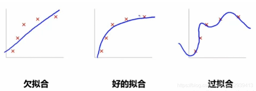
解决过拟合的方法:降低数据量,正则化(L1,L2),Dropout(把其中的一些神经元去掉只用部分神经元去构建神经网络)
解决欠拟合的方法:增加训练数据,优化算法
8.2 交叉验证
更详细参考:交叉验证(Cross Validation)
数据集可划分为三类:
- 训练集——用于训练的数据集
- 评估验证集——用于训练过程中进行评估反馈的集合,有时候也参与训练集
- 测试集——用于验收训练结果
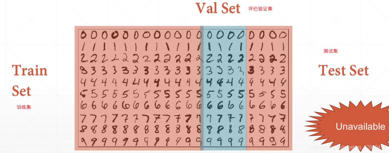
# 分为三个集合db_train、 db_val、 db_test
(x,y),(xtest,y_test)=datasets.mnist.load_data()
xtrain,xval=tf.split(x,numor_size_splits=[50000,10000])
y_train,y_val=tf.split(y,num_or_size_splits=[50000,10000])
db_train=tf.data.Dataset.from_tensor_slices((x_train,y_train))
db_train=db_train.map(preprocess).shuffle(50000).batch(batchsz)
db_val=tf.data.Dataset.from_tensor_slices((x_val,y_val))
db_val=db_val.map(preprocess).shuffle(10000).batch(batchsz)db_test=tf.data.Dataset.from_tensor_slices((x_test,y_test))
db_test=db_test.map(preprocess).batch(batchsz)
# 建立模型
network. compile(optimizer=optimizers. Adam(Lr=0.01), loss=tf. losses. CategoricalCrossentropy(from_logit s=True), metrics=[' accuracy']
# 执行模型
# validation_data=db_val 为评估集合;validation_freq=2为每两个epochs评估一次
network. fit(db_train, epochs=5, validation_data=db_val, validation_freq=2)
# 测试
print(' Test performance:1)
network. evaluate(db_test)
进一步可以使用交叉验证方法,即将数据集分为训练集和测试集,其中训练集均分为N份,每个epochs随机采用N-1份作为训练集,剩余一份作为评估验证集,实现交叉验证。

第一种编程表达方式(原始):
for epoch in range(500): idx=tf. range(60000)
idx=tf. random. shuffle(idx) # 随机打散
xtrain, ytrain=tf. gather(x, idx[:50000]), tf. gather(y, idx[:50000]) # 5/6作为训练集
xval,y_val=tf. gather(x, idx[-10000:]), tf. gather(y, idx[-10000:]) # 1/6作为测试集
db_train=tf. data. Dataset. from_tensor_slices((x_train,y_train))
db_train=db_train. map(preprocess). shuffle(50000). batch(batchsz)
db_val=tf. data. Dataset. from_tensor_slices((x_val,y_val))
db_val=db_val. map(preprocess). shuffle(10000). batch(batchsz)
# training…
# evalutation..
第二种编程表达方式(封装):
# 其中validation_split=0.1表示评估验证集占1/10,验证方式为交叉验证;validation_freq=2为每两个epochs评估一次
network.fit(db_train_val,epochs=6,validation_split=0.1,validation_freq=2)
8.3 正则化(Regularization)
简单来说,正则化是一种为了减小测试误差的行为(有时候会增加训练误差)。我们在构造机器学习模型时,最终目的是让模型在面对新数据的时候,可以有很好的表现。当你用比较复杂的模型比如神经网络,去拟合数据时,很容易出现过拟合现象(训练集表现很好,测试集表现较差),这会导致模型的泛化能力下降,这时候,我们就需要使用正则化,降低模型的复杂度。
作者:Zero黑羽枫 链接:https://www.jianshu.com/p/569efedf6985
正则化一般分为:
- L1范数正则化——更适用于特征选择
- L2范数正则化——更适用于防止模型过拟合
- 详细原理参考:机器学习中的正则化(Regularization)
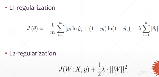
l2_model=keras. models. Sequential([
	keras. layers. Dense(16, kernel_regularizer=keras. regularizers.l2(0.001),
		activation=tf. nn. relu, input_shape=(NUM_WORDS,)),
	keras. layers. Dense(16, kerne l_regularizer=keras. regularizers.L2(0.001),
		activation=tf. nn. relu),
	keras. layers. Dense(1, activation=tf. nn. sigmoid)
])
以上代码只是对W进行了正则化
kernel_regularizer=keras. regularizers.l2(0.001)表示对kernel,即W进行正则化,l2表示L2范数正则化,0.001表示λ=0.001
更加灵活的正则化代码:
for step, (x,y) in enumerate(db):

    with tf.GradientTape() as tape:
  		 ......
        loss = tf.reduce_mean(tf.losses.categorical_crossentropy(y_onehot, out, from_logits=True))

        # --------------正则化惩罚项--------------
        loss_regularization = []
        for p in network.trainable_variables:
            loss_regularization.append(tf.nn.l2_loss(p)) # l2范数正则化
        loss_regularization = tf.reduce_sum(tf.stack(loss_regularization))
        # --------------正则化惩罚项--------------
        loss = loss + 0.0001 * loss_regularization


    grads = tape.gradient(loss, network.trainable_variables)
    optimizer.apply_gradients(zip(grads, network.trainable_variables))
8.4 动量与学习率
8.4.1 动量梯度下降
动量梯度下降法是对梯度下降法的改良版本,通常来说优化效果好于梯度下降法。
普通的梯度下降法每次更新仅与当前梯度值相关,并不涉及之前的梯度。而动量梯度下降法使用指数加权平均之后梯度代替原梯度进行参数更新,将之前的梯度影响考虑在内。
更详细参考:动量梯度下降法(gradient descent with momentum)
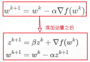
以下代码中的momentum就是表示之前的梯度影响有多大,0.9表示 之前的梯度影响:现在梯度为 9:1
optimizer=SGD(learning_rate=0.02, momentum=0.9) # 随机梯度下降
optimizer=RMSprop(learning_rate=0.02, momentum=0.9)# AdaGrad算法的一种改进
optimizer=Adma(learning_rate=0.02, beta_1=0.9, beta_2=0.999) # 自适应时刻估计方法,momentum也采用自适应,无需设置
各种神经网络优化算法参考:
8.4.2 学习率调整
直接在代码中实现调整,一般设置为随着训练的进行学习率逐渐减小
Adaptive learning rate:
optimizer=SGD(learning_rate=0.2)
for epoch in range(100):
# get loss
# change learning rate
optimizer. learning_rate=0.2*(100-epoch)/100
# update weights
8.5 其他训练Tricks
8.5.1 Early Stopping
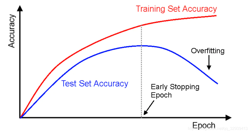
在测试结果最好的时候停下并保存训练参数,称为早停法
详细内容参考:深度学习技巧之Early Stopping(早停法)
8.5.2 Dropout
dropout是指在深度学习网络的训练过程中,对于神经网络单元,按照一定的概率将其暂时从网络中丢弃。
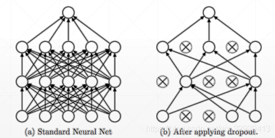
主要作用是减小训练负担,避免过拟合现象
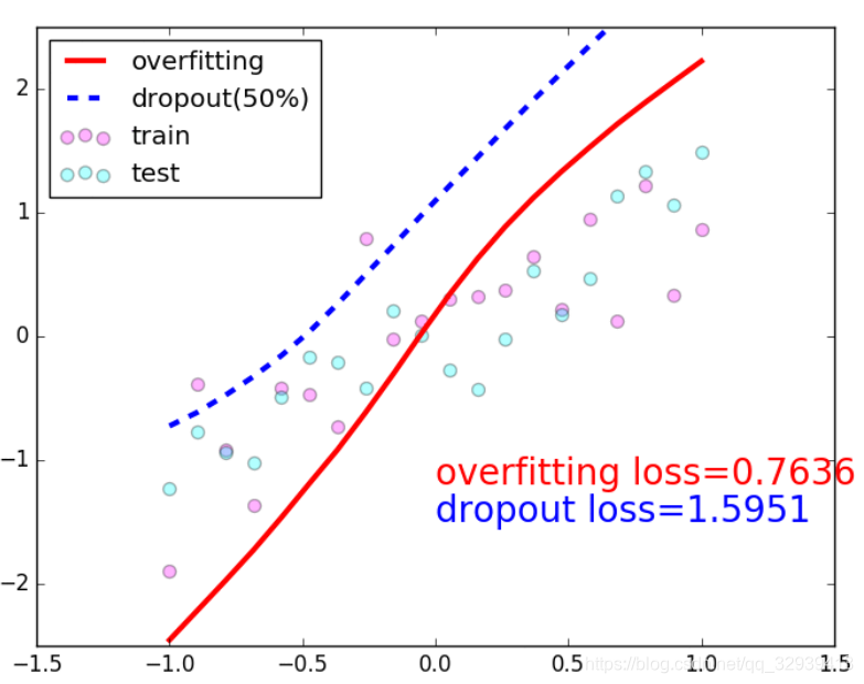
API:
layer.Dropout(rate)tf.nn.dropout(x, rate)
CODE:
network=Sequential([ layers. Dense(256, activation=' relu'),
layers. Dropout(0.5),#0.5 rate to drop
layers. Dense(128, activation=' relu'),
layers. Dropout(0.5),#0.5 rate to drop
layers. Dense(64, activation=' relul),
Layers. Dense(32, activation=' relul),
layers. Dense(10)])
在训练过程中要注意training=True而测试或者评估验证时training=False
for step,(x,y) in enumerate(db): with tf. GradientTape() as tape:
#[b,28,28]=>[b,784]
x=tf. reshape(x,(-1,28*28))
#[b,784]=>[b,10]
out=network(x, training=True)
# test out=network(x, training=False)
更详细参考:深度学习网络大杀器之Dropout——深入解析Dropout
8.5.3 【易混淆解释】Stochastic not random!
类似于按照某分布随机抽样求均值,再进行梯度更新,而不是随机的方向;
随机梯度下降法减小了计算开销。
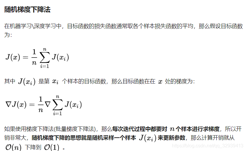


 559
559


 被折叠的 条评论
为什么被折叠?
被折叠的 条评论
为什么被折叠?
 到【灌水乐园】发言


