Pytorch入门学习

引言

Pytorch越来越成为深度学习的主流框架。为什么它这么受欢迎呢？因为Pytorch可以显著加快完成机器学习任务的速度。那它是什么原理呢？那就要从硬件说起啦。
近年来我们能训练更强大更复杂的模型，得益于计算机处理器的性能一直在提升，比如用含有100个神经元的多层感知机实现一个手写体识别任务，这个最简单的模型就包含将近80000个参数，如果想再加些隐藏层层数，参数将会爆炸式增长。那这些参数用什么处理呢？一般用显卡GPU，因为它的内核数是CPU的几百倍，浮点计算量是CPU的几十倍。但问题是，利用GPU比较复杂，需要一些特殊软件包，如CUDA，OpenCL，来允许对GPU编程。所以，为了更方便的利用GPU，人们开发了pytorch。

Pytorch 基本概念

继2016年由Facebook开发及发布，和2018年推行1.0版本之后，Pytorch已成为最受欢迎的深度学习框架之一。根据修改后的BSD许可，Pytorch是免费开源的。Pytorch可以在CPU，GPU，XLA设备（如TPU）上运行，但是只有GPU和XLA才能发挥pytorch的最大性能。Pytorch是基于Torch库开发的，顾名思义，Pytorch的开发重点就是Python接口。
Pytorch建立在由一组节点构成的计算图基础之上。每个节点代表一个操作，该操作可能有0个或多个输入输出。Pytorch提供一个命令式编程环境，用于评估操作、执行计算并立即返回具体值。因此，Pytorch中的计算图是隐式定义的，并不是在计算之前预先构建的。

下面了解基本概念，以及学习常用的几个函数。

张量（Tensor）

在数学上，张量可以理解为标量（0阶张量）、向量（1阶张量）、矩阵（2阶张量）的泛化。PyTorch 张量(Tensor)，张量是PyTorch最基本的操作对象，英文名称为Tensor，它表示的是一个多维的矩阵。比如零维是一个点，一维就是向量，二维就是一般的矩阵，多维就相当于一个多维的数组，这和numpy的数组是对应的，而且 Pytorch 的 Tensor 可以和 numpy 的ndarray相互转换，唯一不同的是Pytorch可以在GPU上运行，且张量经过优化，可用于自动微分，而numpy的 ndarray 只能在CPU上运行。

常用的不同数据类型的 Tensor 如下:

• 32位浮点型 torch.FloatTensor
• 64位浮点型 torch.DoubleTensor
• 16位整型 torch.ShortTensor
• 32位整型 torch.IntTensor
• 64位整型 torch.LongTensor

变量（Variable）

Variable，也就是变量，这个在numpy里面是没有的，是神经网络计算图里特有的一个概念，就是Variable提供了自动求导的功能，之前如果了解Tensorflow的读者应该清楚神经网络在做运算的时候需要先构造一个计算图谱，然后在里面运行前向传播和反向传播。
Variable和Tensor本质上没有区别，不过Variable会被放入一个计算图中，然后进行前向传播，反向传播，自动求导。
首先Variable是在torch.autograd.Variable中，要将一个tensor变成Variable也非常简单，比如想让一个tensor a变成Variable，只需要Variable(a)就可以了。Variable的属性如下：

Variable 有三个比较重要的组成属性：data、grad和grad_fn。通过data可以取出 Variable 里面的tensor数值，grad_fn表示的是得到这个Variable的操作。比如通过加减还是乘除来得到的，最后grad是这个Variable的反向传播梯度。
构建Variable，要注意得传入一个参数requires_grad=True，这个参数表示是否对这个变量求梯度，默认的是False，也就是不对这个变量求梯度，这里我们希望得到这些变量的梯度，所以需要传入这个参数。
y.backward()，这一行代码就是所谓的自动求导，这其实等价于y.backward(torch.FloatTensor([1]))，只不过对于标量求导里面的参数就可以不写了，自动求导不需要你再去明确地写明哪个函数对哪个函数求导，直接通过这行代码就能对所有的需要梯度的变量进行求导，得到它们的梯度，然后通过x.grad可以得到x的梯度。
矩阵求导，相当于给出了一个三维向量去做运算，这时候得到的结果y就是一个向量，这里对这个向量求导就不能直接写成y.backward()，这样程序就会报错的。这个时候需要传入参数声明，比如y.backward(troch.FloatTensor([1, 1, 1]))，这样得到的结果就是它们每个分量的梯度，或者可以传入y.backward(torch.FloatTensor([1, 0.1, 0.01]))，这样得到的梯度就是它们原本的梯度分别乘上1, 0.1 和 0.01。

数据集（dataset）

数据读取和预处理是进行机器学习的首要操作，PyTorch提供了很多方法来完成数据的读取和预处理。本文介绍 Dataset，TensorDataset，DataLoader，ImageFolder的简单用法。

torch.utils.data.Dataset

Dataset类：
PyTorch 读取数据，主要是通过 Dataset 类，所以先简单了解一下 Dataset 类。Dataset类作为所有的 datasets 的基类存在，所有的 datasets 都需要继承它！
Dataset源码：

class Dataset(object):
"""An abstract class representing a Dataset.
All other datasets should subclass it. All subclasses should override
``__len__``, that provides the size of the dataset, and ``__getitem__``,
supporting integer indexing in range from 0 to len(self) exclusive.
"""
	def __getitem__(self, index):
		raise NotImplementedError
	def __len__(self):
		raise NotImplementedError
	def __add__(self, other):
		return ConcatDataset([self, other])

这里重点看 getitem 函数，getitem（get获取item每个数据） 接收一个 index，然后返回图片数据和标签，这个index 通常指的是一个 list 的index，这个 list 的每个元素就包含了图片数据的路径和标签信息。

然而，如何制作这个 list 呢? 通常的方法是将图片的路径和标签信息存储在一个 txt中，然后从该 txt 中读取。
那么读取自己数据的基本流程就是：
1.制作存储了图片的路径和标签信息的 txt
2.将这些信息转化为 list，该 list 每一个元素对应一个样本
3.通过 getitem 函数，读取数据和标签，并返回数据和标签

在训练代码里是感觉不到这些操作的，只会看到通过DataLoader 就可以获取一个batch 的数据。

因此，要让 PyTorch 能读取自己的数据集，只需要两步：

1. 制作图片数据的索引
2. 构建 Dataset 子类

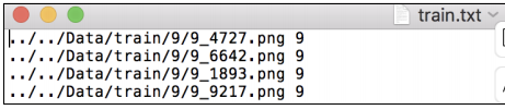
第一步：制作图片数据的索引
就是读取图片路径，标签，保存到 txt 文件中，这里注意格式就好。特别注意的是，txt 中的路径，是以训练时的那个 py 文件所在的目录为工作目录，所以这里需要提前算好相对路径！
txt 中是这样的：

第二步：建 Dataset 子类：
通常，一般存在两个或多个张量，比如一个特征张量csv_data，一个标签张量txt_data，那就需要构建一个联合数据集。

torch.utils.data.Dataset是代表这一数据的抽象类。你可以自己定义你的数据类，继承和重写这个抽象类，非常简单，只需要定义_ len 和 _ getitem_这个两个函数：

from torch.utils.data import Dataset
import pandas as pd

class myDataset(Dataset):
    def __init__(self,csv_file,txt_file,root_dir, other_file):# 初始化方法，如读取数据，加载文件，过滤数据等
        self.csv_data = pd.read_csv(csv_file)
        with open(txt_file,'r') as f:
            data_list = f.readlines()
        self.txt_data = data_list
        self.root_dir = root_dir

    def __len__(self):
        return len(self.csv_data)

    def __gettime__(self,idx): # 返回给定索引对应样本
        data = (self.csv_data[idx],self.txt_data[idx])
        return data

通过上面的方式，可以定义我们需要的数据类，可以通过迭代的方式来获取每一个数据，但这样很难实现取batch，shuffle或者是多线程去读取数据。

torch.utils.data.TensorDataset

torch.utils.data.TensorDataset 继承自 Dataset，新版把之前的data_tensor和target_tensor去掉了，输入变成了可变参数，也就是我们平常使用*args。

from torch.utils.data import TensorDataset

# 原版使用方法
train_dataset = TensorDataset(data_tensor=x, target_tensor=y)

# 新版使用方法
train_dataset = TensorDataset(csv_data,txt_data)

for i in train_dataset:
	print(i[0],1[1]) 

使用 TensorDataset 的方法可以参考下面的例子：

import torch
from torch.utils.data.DataLoader import DataLoader
from torch.utils.data import TensorDataset

BATCH_SIZE = 5

x = torch.linspace(1, 10, 10)
y = torch.linspace(10, 1, 10)

torch_dataset = TensorDataset(x, y)
loader = DataLoader(
    dataset=torch_dataset,
    batch_size=BATCH_SIZE,
    shuffle=True,
    num_workers=0,
)

for epoch in range(3):
    for step, (batch_x, batch_y) in enumerate(loader):
        print('Epoch: ', epoch, '| Step: ', step, '| batch x: ', batch_x.numpy(), '| batch y: ', batch_y.numpy())

执行结果：

数据中的行被shuffle打乱，但x和y之间的对应关系没有乱。

torch.utils.data.DataLoader

如果数据已经以张量、Python列表或Numpy数组的结构存储，则可使用 torch.utils.data.DataLoader类创建数据集加载器。该数据集将返回DataLoader的一个对象，可以使用它来遍历数据集中的各个元素。
示例：用包含0-5的列表创建一个数据集

from torch.utils.data.DataLoader import DataLoader

t = torch.arrange(6,dtype=torch.float32)
data = DataLoader(t)

# 可以看看data里的每个元素
for i in data:
	print(i)

如果想用这个数据创建大小为3的批数据，可以设置batch_size，drop_last为可选参数，默认为False，为True时表示当张量中的元素数量不能被批处理大小整除时，删除最后一个不完整的批。

data = DataLoader(t, batch_size=3, drop_last=false)

还有其他参数

dataiter = DataLoader(myDataset,batch_size=32,shuffle=True,collate_fn=defaulf_collate)

其中的参数都很清楚，只有 collate_fn 是标识如何取样本的，我们可以定义自己的函数来准确地实现想要的功能，默认的函数在一般情况下都是可以使用的。
需要注意的是，Dataset类只相当于一个打包工具，包含了数据的地址。真正把数据读入内存的过程是由Dataloader进行批迭代输入的时候进行的。

源码中DataLoader：

class DataLoader(object):
    r"""
    Data loader. Combines a dataset and a sampler, and provides an iterable over
    the given dataset.数据加载。结合数据集和采样器，并提供给定数据集上的可迭代对象。

    The :class:`~torch.utils.data.DataLoader` supports both map-style and
    iterable-style datasets with single- or multi-process loading, customizing
    loading order and optional automatic batching (collation) and memory pinning.
    类:'~ torch.utils.data.DataLoader' 支持地图风格和可迭代风格的数据集与单或多进程加载，
    自定义加载顺序和可选的自动批处理(整理)和内存固定。
    
    See :py:mod:`torch.utils.data` documentation page for more details.

    Arguments:
        dataset (Dataset): dataset from which to load the data.
        batch_size (int, optional): how many samples per batch to load
            (default: ``1``).
        shuffle (bool, optional): set to ``True`` to have the data reshuffled
            at every epoch (default: ``False``).
        sampler (Sampler, optional): defines the strategy to draw samples from
            the dataset. If specified, :attr:`shuffle` must be ``False``.
        batch_sampler (Sampler, optional): like :attr:`sampler`, but returns a batch of
            indices at a time. Mutually exclusive with :attr:`batch_size`,
            :attr:`shuffle`, :attr:`sampler`, and :attr:`drop_last`.
        num_workers (int, optional): how many subprocesses to use for data
            loading. ``0`` means that the data will be loaded in the main process.
            (default: ``0``)
        collate_fn (callable, optional): merges a list of samples to form a
            mini-batch of Tensor(s).  Used when using batched loading from a
            map-style dataset.
        pin_memory (bool, optional): If ``True``, the data loader will copy Tensors
            into CUDA pinned memory before returning them.  If your data elements
            are a custom type, or your :attr:`collate_fn` returns a batch that is a custom type,
            see the example below.
        drop_last (bool, optional): set to ``True`` to drop the last incomplete batch,
            if the dataset size is not divisible by the batch size. If ``False`` and
            the size of dataset is not divisible by the batch size, then the last batch
            will be smaller. (default: ``False``)
        timeout (numeric, optional): if positive, the timeout value for collecting a batch
            from workers. Should always be non-negative. (default: ``0``)
        worker_init_fn (callable, optional): If not ``None``, this will be called on each
            worker subprocess with the worker id (an int in ``[0, num_workers - 1]``) as
            input, after seeding and before data loading. (default: ``None``)


    .. warning:: If the ``spawn`` start method is used, :attr:`worker_init_fn`
                 cannot be an unpicklable object, e.g., a lambda function. See
                 :ref:`multiprocessing-best-practices` on more details related
                 to multiprocessing in PyTorch.

    .. note:: ``len(dataloader)`` heuristic is based on the length of the sampler used.
              When :attr:`dataset` is an :class:`~torch.utils.data.IterableDataset`,
              an infinite sampler is used, whose :meth:`__len__` is not
              implemented, because the actual length depends on both the
              iterable as well as multi-process loading configurations. So one
              should not query this method unless they work with a map-style
              dataset. See `Dataset Types`_ for more details on these two types
              of datasets.
    """

    __initialized = False

    def __init__(self, dataset, batch_size=1, shuffle=False, sampler=None,
                 batch_sampler=None, num_workers=0, collate_fn=None,
                 pin_memory=False, drop_last=False, timeout=0,
                 worker_init_fn=None, multiprocessing_context=None):
        torch._C._log_api_usage_once("python.data_loader")

        if num_workers < 0:
            raise ValueError('num_workers option should be non-negative; '
                             'use num_workers=0 to disable multiprocessing.')

        if timeout < 0:
            raise ValueError('timeout option should be non-negative')

        self.dataset = dataset
        self.num_workers = num_workers
        self.pin_memory = pin_memory
        self.timeout = timeout
        self.worker_init_fn = worker_init_fn
        self.multiprocessing_context = multiprocessing_context

        # Arg-check dataset related before checking samplers because we want to
        # tell users that iterable-style datasets are incompatible with custom
        # samplers first, so that they don't learn that this combo doesn't work
        # after spending time fixing the custom sampler errors.
        if isinstance(dataset, IterableDataset):
            self._dataset_kind = _DatasetKind.Iterable
            # NOTE [ Custom Samplers and `IterableDataset` ]
            #
            # `IterableDataset` does not support custom `batch_sampler` or
            # `sampler` since the key is irrelevant (unless we support
            # generator-style dataset one day...).
            #
            # For `sampler`, we always create a dummy sampler. This is an
            # infinite sampler even when the dataset may have an implemented
            # finite `__len__` because in multi-process data loading, naive
            # settings will return duplicated data (which may be desired), and
            # thus using a sampler with length matching that of dataset will
            # cause data lost (you may have duplicates of the first couple
            # batches, but never see anything afterwards). Therefore,
            # `Iterabledataset` always uses an infinite sampler, an instance of
            # `_InfiniteConstantSampler` defined above.
            #
            # A custom `batch_sampler` essentially only controls the batch size.
            # However, it is unclear how useful it would be since an iterable-style
            # dataset can handle that within itself. Moreover, it is pointless
            # in multi-process data loading as the assignment order of batches
            # to workers is an implementation detail so users can not control
            # how to batchify each worker's iterable. Thus, we disable this
            # option. If this turns out to be useful in future, we can re-enable
            # this, and support custom samplers that specify the assignments to
            # specific workers.
            if shuffle is not False:
                raise ValueError(
                    "DataLoader with IterableDataset: expected unspecified "
                    "shuffle option, but got shuffle={}".format(shuffle))
            elif sampler is not None:
                # See NOTE [ Custom Samplers and IterableDataset ]
                raise ValueError(
                    "DataLoader with IterableDataset: expected unspecified "
                    "sampler option, but got sampler={}".format(sampler))
            elif batch_sampler is not None:
                # See NOTE [ Custom Samplers and IterableDataset ]
                raise ValueError(
                    "DataLoader with IterableDataset: expected unspecified "
                    "batch_sampler option, but got batch_sampler={}".format(batch_sampler))
        else:
            self._dataset_kind = _DatasetKind.Map

        if sampler is not None and shuffle:
            raise ValueError('sampler option is mutually exclusive with '
                             'shuffle')

        if batch_sampler is not None:
            # auto_collation with custom batch_sampler
            if batch_size != 1 or shuffle or sampler is not None or drop_last:
                raise ValueError('batch_sampler option is mutually exclusive '
                                 'with batch_size, shuffle, sampler, and '
                                 'drop_last')
            batch_size = None
            drop_last = False
        elif batch_size is None:
            # no auto_collation
            if shuffle or drop_last:
                raise ValueError('batch_size=None option disables auto-batching '
                                 'and is mutually exclusive with '
                                 'shuffle, and drop_last')

        if sampler is None:  # give default samplers
            if self._dataset_kind == _DatasetKind.Iterable:
                # See NOTE [ Custom Samplers and IterableDataset ]
                sampler = _InfiniteConstantSampler()
            else:  # map-style
                if shuffle:
                    sampler = RandomSampler(dataset)
                else:
                    sampler = SequentialSampler(dataset)

        if batch_size is not None and batch_sampler is None:
            # auto_collation without custom batch_sampler
            batch_sampler = BatchSampler(sampler, batch_size, drop_last)

        self.batch_size = batch_size
        self.drop_last = drop_last
        self.sampler = sampler
        self.batch_sampler = batch_sampler

        if collate_fn is None:
            if self._auto_collation:
                collate_fn = _utils.collate.default_collate
            else:
                collate_fn = _utils.collate.default_convert

        self.collate_fn = collate_fn
        self.__initialized = True

    @property
    def multiprocessing_context(self):
        return self.__multiprocessing_context

    @multiprocessing_context.setter
    def multiprocessing_context(self, multiprocessing_context):
        if multiprocessing_context is not None:
            if self.num_workers > 0:
                if not multiprocessing._supports_context:
                    raise ValueError('multiprocessing_context relies on Python >= 3.4, with '
                                     'support for different start methods')

                if isinstance(multiprocessing_context, string_classes):
                    valid_start_methods = multiprocessing.get_all_start_methods()
                    if multiprocessing_context not in valid_start_methods:
                        raise ValueError(
                            ('multiprocessing_context option '
                             'should specify a valid start method in {}, but got '
                             'multiprocessing_context={}').format(valid_start_methods, multiprocessing_context))
                    multiprocessing_context = multiprocessing.get_context(multiprocessing_context)

                if not isinstance(multiprocessing_context, python_multiprocessing.context.BaseContext):
                    raise ValueError(('multiprocessing_context option should be a valid context '
                                      'object or a string specifying the start method, but got '
                                      'multiprocessing_context={}').format(multiprocessing_context))
            else:
                raise ValueError(('multiprocessing_context can only be used with '
                                  'multi-process loading (num_workers > 0), but got '
                                  'num_workers={}').format(self.num_workers))

        self.__multiprocessing_context = multiprocessing_context

    def __setattr__(self, attr, val):
        if self.__initialized and attr in ('batch_size', 'batch_sampler', 'sampler', 'drop_last', 'dataset'):
            raise ValueError('{} attribute should not be set after {} is '
                             'initialized'.format(attr, self.__class__.__name__))

        super(DataLoader, self).__setattr__(attr, val)

    def __iter__(self):
        if self.num_workers == 0:
            return _SingleProcessDataLoaderIter(self)
        else:
            return _MultiProcessingDataLoaderIter(self)

    @property
    def _auto_collation(self):
        return self.batch_sampler is not None

    @property
    def _index_sampler(self):
        # The actual sampler used for generating indices for `_DatasetFetcher`
        # (see _utils/fetch.py) to read data at each time. This would be
        # `.batch_sampler` if in auto-collation mode, and `.sampler` otherwise.
        # We can't change `.sampler` and `.batch_sampler` attributes for BC
        # reasons.
        if self._auto_collation:
            return self.batch_sampler
        else:
            return self.sampler

    def __len__(self):
        return len(self._index_sampler)  # with iterable-style dataset, this will error

torchvision.datasets.ImageFolder

另外在torchvison这个包中还有一个更高级的有关于计算机视觉的数据读取类：ImageFolder，主要功能是处理图片，且要求图片是下面这种存放形式：
root/dog/xxx.png
root/dog/xxy.png
root/dog/xxz.png

root/cat/123.png
root/cat/asd/png
root/cat/zxc.png

之后这样来调用这个类:

from torchvision.datasets import ImageFolder

dset = ImageFolder(root='root_path', transform=None, loader=default_loader)

其中 root 需要是根目录，在这个目录下有几个文件夹，每个文件夹表示一个类别：transform 和 target_transform 是图片增强，后面我们会详细介绍；loader是图片读取的办法，因为我们读取的是图片的名字，然后通过 loader 将图片转换成我们需要的图片类型进入神经网络。

PyTorch 优化

优化算法就是一种调整模型参数更新的策略，在深度学习和机器学习中，我们常常通过修改参数使得损失函数最小化或最大化。
优化算法分为两大类：
(1) 一阶优化算法
这种算法使用各个参数的梯度值来更新参数，最常用的一阶优化算法是梯度下降。所谓的梯度就是导数的多变量表达式，函数的梯度形成了一个向量场，同时也是一个方向，这个方向上方向导数最大，且等于梯度。梯度下降的功能是通过寻找最小值，控制方差，更新模型参数，最终使模型收敛，网络的参数更新公式如下：

(2) 二阶优化算法
二阶优化算法是用来二阶导数（也叫做Hessian方法）来最小化或最大化损失函数，主要基于牛顿法，但由于二阶导数的计算成本很高，所以这种方法并没有广泛使用。torch.optim是一个实现了各种优化算法的库，多数常见的算法都能直接通过这个包来调用，并且接口具备足够的通用性，使得未来能够集成更加复杂的方法，比如随机梯度下降，以及添加动量的随机梯度下降，自适应学习率等。为了构建一个Optimizer，你需要给它一个包含了需要优化的参数（必须都是Variable对象）的iterable。然后设置optimizer的参数选项，比如学习率，动量等等。

import torch
import torch.utils.data as Data
import torch.nn.functional as F
from torch.autograd import Variable
import matplotlib.pyplot as plt

torch.manual_seed(1)    # reproducible

LR = 0.01
BATCH_SIZE = 32
EPOCH = 12

# fake dataset
x = torch.unsqueeze(torch.linspace(-1, 1, 1000), dim=1)
y = x.pow(2) + 0.1*torch.normal(torch.zeros(*x.size()))

# plot dataset
plt.scatter(x.numpy(), y.numpy())
plt.show()

执行结果如下：

为了对比每一种优化器, 我们给他们各自创建一个神经网络, 但这个神经网络都来自同一个 Net 形式。接下来在创建不同的优化器, 用来训练不同的网络. 并创建一个 loss_func 用来计算误差。几种常见的优化器：SGD, Momentum, RMSprop, Adam。

torch_dataset = Data.TensorDataset(x, y)
loader = Data.DataLoader(dataset=torch_dataset, batch_size=BATCH_SIZE, shuffle=True, num_workers=0,)

# 默认的 network 形式
class Net(torch.nn.Module):
    def __init__(self):
        super(Net, self).__init__()
        self.hidden = torch.nn.Linear(1, 20)   # hidden layer
        self.predict = torch.nn.Linear(20, 1)   # output layer

    def forward(self, x):
        x = F.relu(self.hidden(x))      # activation function for hidden layer
        x = self.predict(x)             # linear output
        return x

# 为每个优化器创建一个 net
net_SGD         = Net()
net_Momentum    = Net()
net_RMSprop     = Net()
net_Adam        = Net()
nets = [net_SGD, net_Momentum, net_RMSprop, net_Adam]

# different optimizers
opt_SGD         = torch.optim.SGD(net_SGD.parameters(), lr=LR)
opt_Momentum    = torch.optim.SGD(net_Momentum.parameters(), lr=LR, momentum=0.8)
opt_RMSprop     = torch.optim.RMSprop(net_RMSprop.parameters(), lr=LR, alpha=0.9)
opt_Adam        = torch.optim.Adam(net_Adam.parameters(), lr=LR, betas=(0.9, 0.99))
optimizers = [opt_SGD, opt_Momentum, opt_RMSprop, opt_Adam]

loss_func = torch.nn.MSELoss()
losses_his = [[], [], [], []]   # 记录 training 时不同神经网络的 loss

for epoch in range(EPOCH):
    print('Epoch: ', epoch)
    for step, (batch_x, batch_y) in enumerate(loader):
        b_x = Variable(batch_x)  # 务必要用 Variable 包一下
        b_y = Variable(batch_y)

        # 对每个优化器, 优化属于他的神经网络
        for net, opt, l_his in zip(nets, optimizers, losses_his):
            output = net(b_x)              # get output for every net
            loss = loss_func(output, b_y)  # compute loss for every net
            opt.zero_grad()                # clear gradients for next train
            loss.backward()                # backpropagation, compute gradients
            opt.step()                     # apply gradients
            l_his.append(loss.item())     # loss recoder

训练和 loss 画图，结果如下:

参数初始化

如一个简单的DNN的生成器：

class dnn_generator(nn.Module):
    
    # Weight Initialization [we initialize weights here]
    def weight_init(self):
        nn.init.xavier_uniform_(self.fc1.weight)
        nn.init.xavier_uniform_(self.fc2.weight)
        nn.init.xavier_uniform_(self.fc3.weight)
        nn.init.xavier_uniform_(self.out.weight)

        nn.init.xavier_uniform_(self.fc1.bias)
        nn.init.xavier_uniform_(self.fc2.bias)
        nn.init.xavier_uniform_(self.fc3.bias)
        nn.init.xavier_uniform_(self.out.bias)

    def __init__(self, G_in, G_out, w1, w2, w3):
        super(dnn_generator, self).__init__()
        
        self.fc1= nn.Linear(G_in, w1)
        self.fc2= nn.Linear(w1, w2)
        self.fc3= nn.Linear(w2, w3)
        self.out= nn.Linear(w3, G_out)

        #self.weight_init()
    
    # Deep neural network [you are passing data layer-to-layer]    
    def forward(self, x):

        x = F.relu(self.fc1(x))
        x = F.relu(self.fc2(x))
        x = F.relu(self.fc3(x))
        x = self.out(x)
        return x

那nn.init中有哪些初始化函数呢？

1.均匀分布

torch.nn.init.uniform_(tensor, a=0, b=1)

服从~U ( a , b )

2.正太分布

torch.nn.init.normal_(tensor, mean=0, std=1)

服从~N(mean, std)

3.常数分布

torch.nn.init.constant_(tensor, val)

初始化整个矩阵为常数val

4.全一分布

torch.nn.init.ones_(tensor)

用全1填充张量

5.全0分布

torch.nn.init.zeros_(tensor)

用全0填充张量

6.Xavier

基本思想是通过网络层时，为了使得网络中信息更好的流动，输入和输出的方差尽可能相等，包括前向传播和后向传播。也就是上面代码用到的。

“Xavier”初始化方法是一种很有效的神经网络初始化方法，方法来源于2010年的一篇论文：《Understanding the difficulty of training deep feedforward neural networks》
具体推导可看这篇博客：
https://blog.csdn.net/shuzfan/article/details/51338178

对于Xavier初始化方式，pytorch提供了uniform和normal两种：

torch.nn.init.xavier_uniform_(tensor, gain=1.0)

均匀分布 ~ U(-a,a )

其中， a的计算公式：

torch.nn.init.xavier_normal_(tensor, gain=1)

正态分布~N(0,std)
其中std的计算公式：

7.kaiming_uniform 分布
Xavier在tanh中表现的很好，但在Relu激活函数中表现的很差，所何凯明提出了针对于Relu的初始化方法。
Delving deep into rectifiers: Surpassing human-level performance on ImageNet classification He, K. et al. (2015)

torch.nn.init.kaiming_uniform_(tensor, a=0, mode='fan_in', nonlinearity='leaky_relu')

该方法的思想是：
在ReLU网络中，假定每一层有一半的神经元被激活，另一半为0，所以，要保持方差不变，只需要在 Xavier 的基础上再除以2。

nn.Sequential和nn.Module

1、nn.Sequential
一个序列容器，用于搭建神经网络的模块被按照被传入构造器的顺序添加到nn.Sequential()容器中。除此之外，一个包含神经网络模块的OrderedDict也可以被传入nn.Sequential()容器中。

使用模板：

# Sequential使用实例

# Using Sequential to create a small model. When `model` is run,
# input will first be passed to `Conv2d(1,20,5)`. The output of
# `Conv2d(1,20,5)` will be used as the input to the first
# `ReLU`; the output of the first `ReLU` will become the input
# for `Conv2d(20,64,5)`. Finally, the output of
# `Conv2d(20,64,5)` will be used as input to the second `ReLU`

model = nn.Sequential(
          nn.Conv2d(1,20,5),
          nn.ReLU(),
          nn.Conv2d(20,64,5),
          nn.ReLU()
        )

# Sequential with OrderedDict使用实例
model = nn.Sequential(OrderedDict([
          ('conv1', nn.Conv2d(1,20,5)),
          ('relu1', nn.ReLU()),
          ('conv2', nn.Conv2d(20,64,5)),
          ('relu2', nn.ReLU())
        ]))

上述两种方法构建出的 model 和 model1 是一样的。

nn.Sequential()的本质作用：
与一层一层的单独调用模块组成序列相比，nn.Sequential() 可以允许将整个容器视为单个模块（即相当于把多个模块封装成一个模块），forward()方法接收输入之后，nn.Sequential()按照内部模块的顺序自动依次计算并输出结果。

这就意味着我们可以利用nn.Sequential() 自定义自己的网络层。

from torch import nn


class net(nn.Module):
    def __init__(self, in_channel, out_channel):
        super(net, self).__init__()
        self.layer1 = nn.Sequential(nn.Conv2d(in_channel, in_channel / 4, kernel_size=1),
                                    nn.BatchNorm2d(in_channel / 4),
                                    nn.ReLU())
        self.layer2 = nn.Sequential(nn.Conv2d(in_channel / 4, in_channel / 4),
                                    nn.BatchNorm2d(in_channel / 4),
                                    nn.ReLU())
        self.layer3 = nn.Sequential(nn.Conv2d(in_channel / 4, out_channel, kernel_size=1),
                                    nn.BatchNorm2d(out_channel),
                                    nn.ReLU())
        
    def forward(self, x):
        x = self.layer1(x)
        x = self.layer2(x)
        x = self.layer3(x)
        
        return x

上边的代码，我们通过nn.Sequential()将卷积层，BN层和激活函数层封装在一个层中，输入x经过卷积、BN和ReLU后直接输出激活函数作用之后的结果。

nn.Sequential()和torch.nn.ModuleList什么区别？
torch.nn.ModuleList只是一个储存网络模块的list，其中的网络模块之间没有连接关系和顺序关系。而nn.Sequential()内的网络模块之间是按照添加的顺序级联的。

使用nn.Sequential()类无法创建具有多个输入、多个输出或多个中间网络分支的复杂模型，因此，我们还需要nn.Module。

2、nn.Module

使用模板：

class 网络名字(nn.Module):
    def __init__(self, 一些定义的参数):
        super(网络名字, self).__init__()
        self.layer1 = nn.Linear(num_input, num_hidden)
        self.layer2 = nn.Sequential(...)
        ...

        定义需要用的网络层

    def forward(self, x): # 定义前向传播
        x1 = self.layer1(x)
        x2 = self.layer2(x)
        x = x1 + x2
        ...
        return x

注意：Module 里面也可以使用 Sequential，同时 Module 非常灵活，具体体现在 forward 中，如何复杂的操作都能直观的在 forward 里面执行

他们搭建的网络什么区别？
我们搭建试试：

class Net(torch.nn.Module):
    def __init__(self, n_feature, n_hidden, n_output):
        super(Net, self).__init__()
        self.hidden = torch.nn.Linear(n_feature, n_hidden)
        self.predict = torch.nn.Linear(n_hidden, n_output)

    def forward(self, x):
        x = F.relu(self.hidden(x))
        x = self.predict(x)
        return x
net1 = Net(1, 10, 1)

net2 = torch.nn.Sequential(
    torch.nn.Linear(1, 10),
    torch.nn.Linear(10, 1)
)

看看什么样子：

print(net1)

Net (
  (hidden): Linear(in_features=1, out_features=10, bias=True)
  (predict): Linear(in_features=10, out_features=1, bias=True)
)

print(net2)

Sequential (
  (0): Linear(in_features=1, out_features=10, bias=True)
  (1): Linear(in_features=10, out_features=1, bias=True)
)

好像差不多

这段代码：

lower_layers = []
net3= nn.Sequential(*lower_layers)
print(net3)

输出：

Sequential()

这个代表什么呢？

inception_layers = []
inception_layers += [nn.Conv2d(1, 128, 3, padding=1)]
inception_layers += [nn.ReLU(True)]
inception_layers += [nn.Conv2d(128, 256, 3, padding=1)]
inception_layers += [nn.ReLU(True)]
inception_layers += [nn.Conv2d(256, 128, 3, padding=1)]
inception_layers += [nn.ReLU(True)]
net4 = nn.Sequential(*inception_layers)
print(net4)

输出：

Sequential(
  (0): Conv2d(1, 128, kernel_size=(3, 3), stride=(1, 1), padding=(1, 1))
  (1): ReLU(inplace=True)
  (2): Conv2d(128, 256, kernel_size=(3, 3), stride=(1, 1), padding=(1, 1))
  (3): ReLU(inplace=True)
  (4): Conv2d(256, 128, kernel_size=(3, 3), stride=(1, 1), padding=(1, 1))

nn.Conv2d

看到一段代码，具体conv2d怎么计算的呢？

        lower_layers = []
        lower_layers += [nn.Conv2d(1, 32, 7, 2, 3)] # Out: 500x20x32
        lower_layers += [nn.ReLU(True)]
        lower_layers += [nn.Conv2d(32, 64, 3, 1, 1)] # Out: 1000x25x64
        lower_layers += [nn.ReLU(True)]
        lower_layers += [nn.MaxPool2d(3, (3,2), 1)] # Out: 500x13x192
        lower_layers += [nn.Conv2d(64, 128, 3, 1, 1)] # Out: 1000x25x192
        lower_layers += [nn.ReLU(True)]
        lower_layers += [nn.MaxPool2d(3, (4,2), 1)] # Out: 500x13x192
        lower_layers += [nn.Conv2d(128, 256, 3, 1, 1)] # Out: 1000x25x192
        lower_layers += [nn.ReLU(True)]
        lower_layers += [nn.MaxPool2d(3, (3,2), 1)] # Out: 500x13x192
        lower_layers += [nn.Conv2d(256, 256, 3, 1, 1)] # Out: 1000x25x192
        lower_layers += [nn.ReLU(True)]

1.函数语法格式

torch.nn.Conv2d(
	in_channels, 
	out_channels, 
	kernel_size, 
	stride=1, 
	padding=0, 
	dilation=1, 
	groups=1, 
	bias=True, 
	padding_mode='zeros', 
	device=None, 
	dtype=None
)

参数解释：

• in_channels：输入的通道数，RGB 图像的输入通道数为 3
• out_channels：输出的通道数
• kernel_size：卷积核的大小，一般我们会使用 5x5、3x3 这种左右两个数相同的卷积核，因此这种情况只需要写 kernel_size = 5这样的就行了。如果左右两个数不同，比如3x5的卷积核，那么写作kernel_size = (3, 5)，注意需要写一个 tuple，而不能写一个 list。
• stride = 1：卷积核在图像窗口上每次平移的间隔，即所谓的步长。
• padding：指图像填充，后面的int型常数代表填充的多少（行数、列数），默认为0。需要注意的是这里的填充包括图像的上下左右，以padding=1为例，若原始图像大小为[32, 32]，那么padding后的图像大小就变成了[34, 34]
• dilation：是否采用空洞卷积，默认为1（不采用）。从中文上来讲，这个参数的意义从卷积核上的一个参数到另一个参数需要走过的距离，那当然默认是1了，毕竟不可能两个不同的参数占同一个地方吧（为0）。更形象和直观的图示可以观察Github上的Dilated convolution animations，展示了dilation=2的情况。
• groups：决定了是否采用分组卷积，groups参数可以参考groups参数详解
• bias：即是否要添加偏置参数作为可学习参数的一个，默认为True。
• padding_mode：即padding的模式，默认采用零填充。

2.计算关系

其中 N 为 batch size，C 为输入通道数，H 为图像高，W 为图像宽。

它们之间的关系为：