随机梯度下降法——python实现

随机梯度下降法——python实现

梯度下降法及题目见此博客

Exercise 3:

题目

Now, we turn to use other optimization methods to get the optimal parameters. Can you use Stochastic Gradient Descent to get the optimal parameters? Plots the training error and the testing error at each K-step iterations (the size of K is set by yourself). Can you analyze the plots and make comparisons to those findings in Exercise 1?
Exercise 3: 现在，我们使用其他方法来获得最优的参数。你是否可以用随机梯度下降法获得最优的参数？请使用随机梯度下降法画出迭代次数（每K次，这里的K你自己设定）与训练样本和测试样本对应的误差的图。比较Exercise 1中的实验图，请总结你的发现。

答案

• 误差

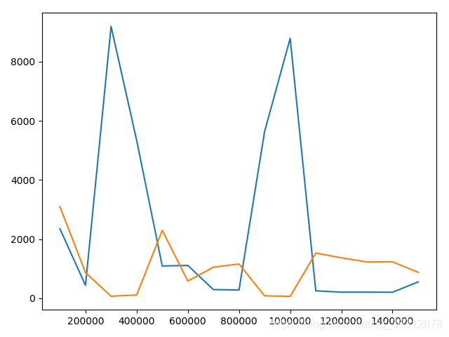
  迭代次数	训练集误差	测试集误差
  100000	2349.4672751626663	3096.2253976063507
  200000	435.2953157918752	867.2532946436027
  300000	9191.947830437808	66.91437740326361
  400000	5340.357593925614	110.47975170582515
  500000	1090.0735267479458	2296.224940582353
  600000	1108.7868485577676	581.28082487602
  700000	292.1925854126944	1050.4866035021282
  800000	278.553496304599	1157.3717939063465
  900000	5638.097793259407	80.34942002974526
  1000000	8791.764070868754	64.02723320568694
  1100000	249.09710616523427	1529.4686707317628
  1200000	204.69153506322482	1366.17101417547
  1300000	205.55798760414544	1227.418573865224
  1400000	202.75800423274228	1228.0429258477968
  1500000	549.766187456897	877.6109789872294

• 误差图
  

• 代码

  import numpy as np
  import math
  import matplotlib.pyplot as plt
  
  
  def loss(train_data, weight, train_real):
      result = np.matmul(train_data, weight.T)
      loss = result - train_real
      losses = pow(loss, 2)
      losses = losses.T
      return losses.sum()
  
  
  def gradient(train_data, weight, train_real):
      num = np.random.randint(0, 50)
      one_train_data = train_data[num]
  
      one_train_real = train_real[num]
      result = np.matmul(one_train_data, weight.T)
      loss = one_train_real - result
      # print (train_real)
      # print (result)
      # print (loss)
      x1 = one_train_data[0]
      x1 = x1
      gradient1 = loss * x1
      x2 = one_train_data[1]
      x2 = x2
      gradient2 = loss * x2
      x3 = train_data.T[2]
      x3 = x3.T
      gradient3 = loss * x3
      return gradient1.T.sum(), gradient2.T.sum(), gradient3.T.sum()
  
  
  filename = "./dataForTraining.txt"
  filename1 = "./dataForTesting.txt"
  
  # input the train data
  read_file = open(filename)
  lines = read_file.readlines()
  
  list_all = []
  list_raw = []
  list_real = []
  for line in lines:
      list1 = line.split()
      for one in list1:
          list_raw.append(float(one))
      list_all.append(list_raw[0:2])
      list_real.append(list_raw[2])
      list_raw = []
  
  for one in list_all:
      one.append(1.0)
  
  train_data = np.array(list_all)
  train_real = np.array(list_real)
  train_real = train_real.T
  
  # input the test data
  read_test = open(filename1)
  test_lines = read_test.readlines()
  
  list_all_test = []
  list_raw_test = []
  list_real_test = []
  for test_line in test_lines:
      another_list = test_line.split()
      for one in another_list:
          list_raw_test.append(float(one))
      list_all_test.append(list_raw_test[0:2])
      list_real_test.append(list_raw_test[2])
      list_raw_test = []
  
  for one in list_all_test:
      one.append(1.0)
  
  train_test_data = np.array(list_all_test)
  train_test_real = np.array(list_real_test)
  train_test_real = train_test_real.T
  
  
  # set the parameter
  weight = np.array([0.0, 0.0, 0.0])
  lr = 0.00015
  x = []
  y = []
  z = []
  
  for num in range(1, 1500001):
      losses = loss(train_data, weight, train_real)
      real_losses = loss(train_test_data, weight, train_test_real)
      gra1, gra2, gra3 = gradient(train_data, weight, train_real)
      gra = np.array([gra1, gra2, gra3])
      weight = weight + (gra * lr)
      # print (losses, real_losses)
      if num % 100000 == 0:
          x.append(num)
          y.append(losses)
          z.append(real_losses)
          print (losses, real_losses)
  
  plt.plot(x, y)
  plt.plot(x, z)
  plt.show()