一文读懂SIFT算法（英文版）

说在前面的话：

本博客转载自 Li Yin 【1】 在medium上写的一篇介绍SIFT的文章，我只是勤劳的搬运工，文章写得真的很易懂，思路清晰,此外，Li Yin还提供了一份论文解读报告。

此外，关于高斯尺度空间（Gaussian Scale Space）部分，我也找到了一份资料，也是通俗易懂，大家可以推导一下加深印象

下面是英文版本的正文：

Scale Invariant Feature Transform (SIFT) Detector and Descriptor

Goal

In this chapter,

• We will learn about the concepts of SIFT algorithm
• We will learn to find SIFT Keypoints and Descriptors.

0. Theory

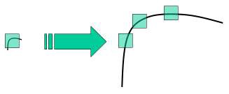
In last couple of chapters, we saw some corner detectors like Harris etc. They are rotation-invariant, which means, even if the image is rotated, we can find the same corners. It is obvious because corners remain corners in rotated image also. But what about scaling? A corner may not be a corner if the image is scaled. For example, check a simple image below. A corner in a small image within a small window is flat when it is zoomed in the same window. So Harris corner is not scale invariant.

So, in 2004, D.Lowe, University of British Columbia, came up with a new algorithm, Scale Invariant Feature Transform (SIFT) in his paper, Distinctive Image Features from Scale-Invariant Keypoints, which extract keypoints and compute its descriptors. (This paper is easy to understand and considered to be best material available on SIFT. So this explanation is just a short summary of this paper).

There are mainly four steps involved in SIFT algorithm. We will see them one-by-one.

Laplacian of Gaussian （LoG）

The Laplacian of Gaussian (LoG) operation goes like this. You take an image, and blur it a little. And then, you calculate second order derivatives on it (or, the “laplacian”). This locates edges and corners on the image. These edges and corners are good for finding keypoints.

But the second order derivative is extremely sensitive to noise. The blur smoothes it out the noise and stabilizes the second order derivative.
The problem is, calculating all those second order derivatives is computationally intensive. So we cheat a bit.

The Con

To generate Laplacian of Guassian images quickly, we use the scale space. We calculate the difference between two consecutive scales. Or, the Difference of Gaussians. Here’s how:

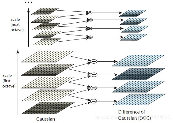
These Difference of Gaussian images are approximately equivalent to the Laplacian of Gaussian. And we’ve replaced a computationally intensive process with a simple subtraction (fast and efficient). Awesome!

These DoG images comes with another little goodie. These approximations are also “scale invariant”. What does that mean?

The Benefits

Just the Laplacian of Gaussian images aren’t great. They are not scale invariant. That is, they depend on the amount of blur you do. This is because of the Gaussian expression. (Don’t panic ? )
$$G(x,y,\sigma )=\frac{1}{2\pi {\sigma }^2}{e}^{-\left(x^2+y^2\right)/2{\sigma }^2}$$

See the σ2 in the demonimator? That’s the scale. If we somehow get rid of it, we’ll have true scale independence. So, if the laplacian of a gaussian is represented like this:
$${\nabla }^{2}G$$
Then the scale invariant laplacian of gaussian would look like this:
$${\sigma }^2{\nabla }^{2}G$$
But all these complexities are taken care of by the Difference of Gaussian operation. The resultant images after the DoG operation are already multiplied by the σ2. Great eh!

Oh! And it has also been proved that this scale invariant thingy produces much better trackable points! Even better!

Side effects

You can’t have benefits without side effects >.<*

You know the DoG result is multiplied with σ2. But it’s also multiplied by another number. That number is (k-1). This is the k we discussed in the previous step.

But we’ll just be looking for the location of the maximums and minimums in the images. We’ll never check the actual values at those locations. So, this additional factor won’t be a problem to us. (Even if you multiply throughout by some constant, the maxima and minima stay at the same location)

Example

Here’s a gigantic image to demonstrate how this difference of Gaussians works.
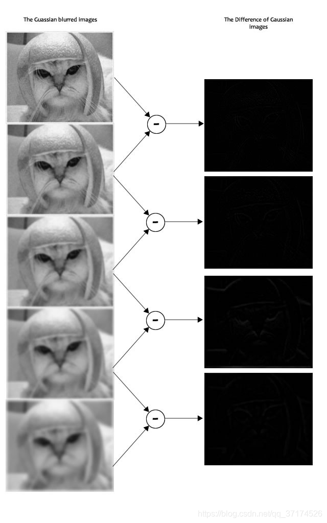In the image, I’ve done the subtraction for just one octave. The same thing is done for all octaves. This generates DoG images of multiple sizes.

1. Scale-space Extrema Detection

From the image above, it is obvious that we can’t use the same window to detect keypoints with different scale. It is OK with small corner. But to detect larger corners we need larger windows. For this, scale-space filtering is used. In it, Laplacian of Gaussian(LoG) is found for the image with various σ values. LoG acts as a blob detector which detects blobs in various sizes due to change in σ. In short, σ acts as a scaling parameter. For eg, in the above image, gaussian kernel with low σ gives high value for small corner while guassian kernel with high σ fits well for larger corner. So, we can find the local maxima across the scale and space which gives us a list of (x,y,σ) values which means there is a potential keypoint at (x,y) at σ scale.

But this LoG is a little costly, so SIFT algorithm uses Difference of Gaussians which is an approximation of LoG. Difference of Gaussian is obtained as the difference of Gaussian blurring of an image with two different σ, let it be σ and kσ. This process is done for different octaves of the image in Gaussian Pyramid. It is represented in below image:

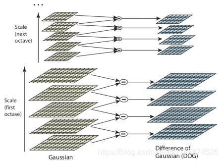
Once this DoG are found, images are searched for local extrema(maxima or minima) over scale and space. For eg, one pixel in an image is compared with its 8 neighbours as well as 9 pixels in next scale and 9 pixels in previous scales. If it is a local extrema, it is a potential keypoint. It basically means that keypoint is best represented in that scale. It is shown in below image:

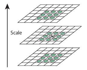
Once this is done, the marked points are the approximate maxima and minima. They are “approximate” because the maxima/minima almost never lies exactly on a pixel. It lies somewhere between the pixel. But we simply cannot access data “between” pixels. So, we must mathematically locate the subpixel location.

Here’s what I mean:

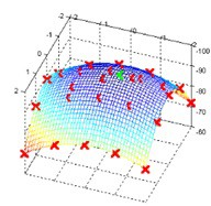
The red crosses mark pixels in the image. But the actual extreme point is the green one.

Find subpixel maxima/minima

Using the available pixel data, subpixel values are generated. This is done by the Taylor expansion of the image around the approximate key point.

Mathematically, it’s like this:
$$D(\mathbf{x})=D+\frac{\partial D^T}{\partial \mathbf{x}}\mathbf{x}+\frac{1}{2}{\mathbf{x}}^{\mathrm{T}}\frac{{\partial }^{2}D}{\partial {\mathbf{x}}^2}\mathbf{x}$$
We can easily find the extreme points of this equation (differentiate and equate to zero). On solving, we’ll get subpixel key point locations. These subpixel values increase chances of matching and stability of the algorithm.

Example

Here’s a result I got from the example image I’ve been using till now:

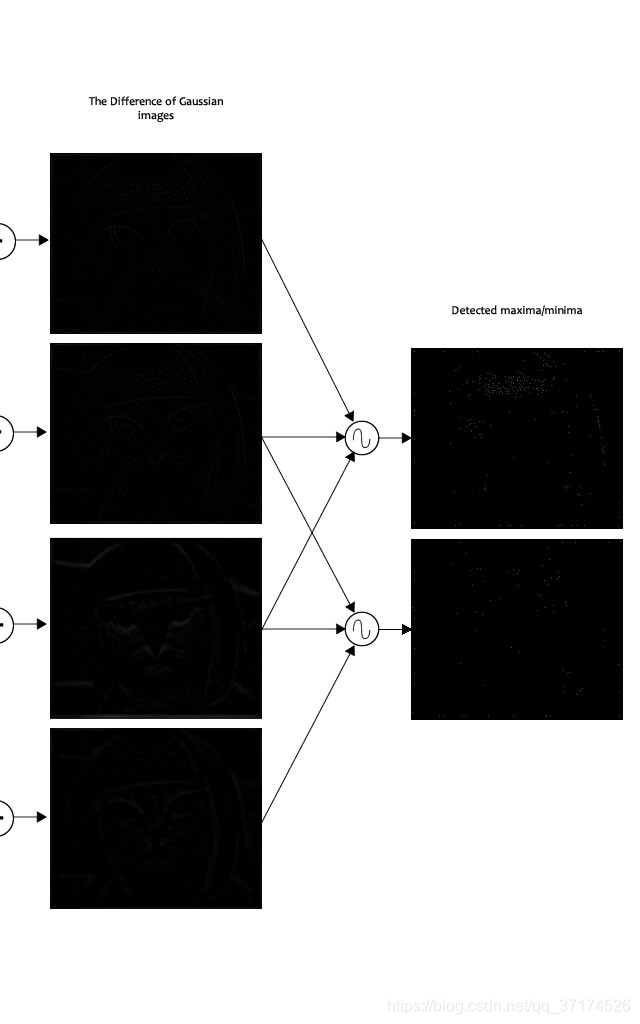
The author of SIFT recommends generating two such extrema images. So, you need exactly 4 DoG images. To generate 4 DoG images, you need 5 Gaussian blurred images. Hence the 5 level of blurs in each octave.

In the image, I’ve shown just one octave. This is done for all octaves. Also, this image just shows the first part of keypoint detection. The Taylor series part has been skipped.

Regarding different parameters, the paper gives some empirical data which can be summarized as, number of octaves = 4, number of scale levels = 5, initial σ=1.6, k=2^(1/2) etc as optimal values.

2. Keypoint Localization

Once potential keypoints locations are found, they have to be refined to get more accurate results. They used Taylor series expansion of scale space to get more accurate location of extrema, and if the intensity at this extrema is less than a threshold value (0.03 as per the paper), it is rejected. This threshold is called contrastThreshold in OpenCV

DoG has higher response for edges, so edges also need to be removed. For this, a concept similar to Harris corner detector is used. They used a 2x2 Hessian matrix (H) to compute the pricipal curvature. We know from Harris corner detector that for edges, one eigen value is larger than the other. So here they used a simple function,

If this ratio is greater than a threshold, called edgeThreshold in OpenCV, that keypoint is discarded. It is given as 10 in paper.

So it eliminates any low-contrast keypoints and edge keypoints and what remains is strong interest points.

3. Orientation Assignment

Now an orientation is assigned to each keypoint to achieve invariance to image rotation. A neigbourhood is taken around the keypoint location depending on the scale, and the gradient magnitude and direction is calculated in that region. An orientation histogram with 36 bins covering 360 degrees is created. (It is weighted by gradient magnitude and gaussian-weighted circular window with σ equal to 1.5 times the scale of keypoint. The highest peak in the histogram is taken and any peak above 80% of it is also considered to calculate the orientation. It creates keypoints with same location and scale, but different directions. It contribute to stability of matching.

4. Keypoint Descriptor

Now keypoint descriptor is created. A 16x16 neighbourhood around the keypoint is taken. It is devided into 16 sub-blocks of 4x4 size. For each sub-block, 8 bin orientation histogram is created. So a total of 128 bin values are available. It is represented as a vector to form keypoint descriptor. In addition to this, several measures are taken to achieve robustness against illumination changes, rotation etc.

5. Keypoint Matching

Keypoints between two images are matched by identifying their nearest neighbours. But in some cases, the second closest-match may be very near to the first. It may happen due to noise or some other reasons. In that case, ratio of closest-distance to second-closest distance is taken. If it is greater than 0.8, they are rejected. It eliminaters around 90% of false matches while discards only 5% correct matches, as per the paper.

So this is a summary of SIFT algorithm. For more details and understanding, reading the original paper is highly recommended. Remember one thing, this algorithm is patented. So this algorithm is included in the opencv contrib repo.

SIFT in OpenCV

So now let’s see SIFT functionalities available in OpenCV. Let’s start with keypoint detection and draw them. First we have to construct a SIFT object. We can pass different parameters to it which are optional and they are well explained in docs.

import cv2
import numpy as np

img = cv2.imread(‘home.jpg’)
gray= cv2.cvtColor(img,cv2.COLOR_BGR2GRAY)

sift = cv2.xfeatures2d.SIFT_create()
kp = sift.detect(gray,None)

img=cv2.drawKeypoints(gray,kp)

cv2.imwrite(‘sift_keypoints.jpg’,img)

sift.detect() function finds the keypoint in the images. You can pass a mask if you want to search only a part of image. Each keypoint is a special structure which has many attributes like its (x,y) coordinates, size of the meaningful neighbourhood, angle which specifies its orientation, response that specifies strength of keypoints etc.

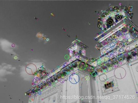
OpenCV also provides cv2.drawKeyPoints() function which draws the small circles on the locations of keypoints. If you pass a flag, cv2.DRAW_MATCHES_FLAGS_DRAW_RICH_KEYPOINTS to it, it will draw a circle with size of keypoint and it will even show its orientation. See below example.

• img=cv2.drawKeypoints(gray,kp,flags=cv2.DRAW_MATCHES_FLAGS_DRAW_RICH_KEYPOINTS)
• cv2.imwrite(‘sift_keypoints.jpg’,img)
  See the two results below image:
  
  Now to calculate the descriptor, OpenCV provides two methods.

  • Since you already found keypoints, you can call sift.compute() which
    computes the descriptors from the keypoints we have found. Eg: kp,des
    = sift.compute(gray,kp)

  • If you didn’t find keypoints, directly find keypoints and descriptors
    in a single step with the function, sift.detectAndCompute().

We will see the second method:

• sift = cv2.xfeatures2d.SIFT_create()
• kp, des = sift.detectAndCompute(gray,None)

Here kp will be a list of keypoints and des is a numpy array of shape Number_of_Keypoints×128.

So we got keypoints, descriptors etc. Now we want to see how to match keypoints in different images. That we will learn in coming chapters.

References

【1】Li Yin, SIFT Detector and Descriptor, https://medium.com/lis-computer-vision-blogs/scale-invariant-feature-transform-sift-detector-and-descriptor-14165624a11, 2018.
【2】David G. Lowe，Distinctive Image Features from Scale-Invariant Keypoints，2004