plt.pcolormesh绘制分类图

最新推荐文章于 2024-05-28 07:49:48 发布

鹏大大大

最新推荐文章于 2024-05-28 07:49:48 发布

阅读量8k

点赞数 3

分类专栏： Python 文章标签： python plt.pcolormesh

Python 专栏收录该内容

62 篇文章 7 订阅

订阅专栏

# -*- coding: utf-8 -*-

'''
多元分类：逻辑回归分类器 并绘制pcolormesh伪彩图
sklearn.linear_model.LogisticRegression(
        solver='liblinear',
        C=正则强度)
'''
# pcolormesh(x, y, c=d, cmap='jet') cmap:渐变色映射

plt.pcolormesh(...):

    a = np.array([1, 2, 3])
    b = np.array([-1, -2, -3, -4])

    a.shape, b.shape
    Out[55]: ((3,), (4,))

    c = np.meshgrid(a, b); c       # c is a 'list', not 'numpy.array'
    Out[57]:                       # c[0]：沿行(axis=0)广播, 每一行元素跟上一行相同
    [array([[1, 2, 3],             # c[1]：沿列(axis=1)广播, 每一列元素跟上一列相同
            [1, 2, 3],             # (c[0],c[1])组成的坐标点(x,y)将覆盖并形成(1<=x<=3,-4<=y<=-1)区间组成的2*3的矩形
            [1, 2, 3],
            [1, 2, 3]]), 
    array([[-1, -1, -1],
            [-2, -2, -2],
            [-3, -3, -3],
            [-4, -4, -4]])]

    c[0].shape, c[1].shape
    Out[61]: ((4, 3), (4, 3))

    plt.pcolormesh(c[0], c[1], c=...)             # c[0]表示点横坐标，c[1]表示纵坐标
    对样本(c[0], c[1])周围（包括样本所在坐标）的四个坐标点进行着色，C代表着色方案
        # 点(c[0], c[1])所有坐标点如下：
        '''
            ^
            |---1------2------3---->
            |
           -1  (1,-1) (2,-1) (3,-1)
            |
           -2  (1,-2) (2,-2) (3,-2)
            |
           -3  (1,-3) (2,-3) (3,-3)
            |
           -4  (1,-4) (2,-4) (3,-4)
            |
            '''

# -*- coding: utf-8 -*-
"""
Created on Tue Jul 31 16:12:18 2018

@author: Administrator
"""
'''
多元分类：逻辑回归分类器
sklearn.linear_model.LogisticRegression(
        solver='liblinear',
        C=正则强度)
'''

import numpy as np
import matplotlib.pyplot as plt
import sklearn.linear_model as lm

# train_set
x = np.array([
        [4, 7],
        [3.5, 8],
        [3.1, 6.2],
        [0.5, 1],
        [1, 2],
        [1.2, 1.9],
        [4, 2],
        [5.7, 1.5],
        [5.4, 2.2]])                                             # 散点[x,y]
y = np.array([0, 0, 0, 1, 1, 1, 2, 2, 2])                        # 多元分类 3类

# 逻辑回归分类器
model = lm.LogisticRegression(solver='liblinear', C=50)          # C
model.fit(x, y)

plt.figure('Logistic Classification', facecolor='lightgray')
plt.title('Logistic Classification', fontsize=14)
plt.xlabel('x', fontsize=14)
plt.ylabel('y', fontsize=14)
plt.tick_params(labelsize=10)

'''
pcolormesh参数设置：
'''
l, r, h = x[:, 0].min() - 1, x[:, 0].max() + 1, 0.005            # 左边界，右边界，水平方向点间距
b, t, v = x[:, 1].min() - 1, x[:, 1].max() + 1, 0.005            # 下边界，上边界，垂直方向点间距

#print(np.arange(l, r, h).shape, np.arange(b, t, v).shape)       # (1440,) (1800,),shape不同，不能直接作为输入,转为
grid_x = np.meshgrid(np.arange(l, r, h), np.arange(b, t, v))     # (m-array,n-array)--> list(mat(m,n), mat(m,n))

print(grid_x[0])                                                 # x[i, j]  (1800, 1440) <class 'numpy.ndarray'> 
print(grid_x[1])                                                 # y[i, j]  (1800, 1440) <class 'numpy.ndarray'> 
#print(grid_x[1].shape)                                          # (1800, 1440) <class 'numpy.ndarray'>
flat_x = np.c_[grid_x[0].ravel(), grid_x[1].ravel()]             # 保证输入散点的坐标点横纵坐标个数一样
flat_y = model.predict(flat_x)                                   # 输入栅格点阵坐标，模型预测输出的分类
grid_y = flat_y.reshape(grid_x[0].shape)                         # 分类标签：用做pcolormesh栅格着色的依据
print(grid_y)
#[[1 1 1 ... 2 2 2]             # 0, 1, 2 分别代表三种不同颜色
# [1 1 1 ... 2 2 2]
# [1 1 1 ... 2 2 2]
# ...
# [0 0 0 ... 0 0 0]
# [0 0 0 ... 0 0 0]
# [0 0 0 ... 0 0 0]]


# pcolormesh: 伪彩图 pcolormesh(X, Y, C) 
# X,Y均为2-D array,如果为1-D 会自动广播，X和Y构成网格点阵
# X,Y对应位置元素x[i,j]和y[i,j]组成一个坐标点(x[i,j],y[i,j])，对样本周围（包括样本所在坐标）的四
#个坐标点进行着色，C代表着色方案
plt.pcolormesh(grid_x[0], grid_x[1], grid_y, cmap='gray')       # gray_r 与gray的色带相反

plt.scatter(x[:, 0], x[:, 1], c=y, cmap='brg', s=60)            # 颜色映射

这里写图片描述

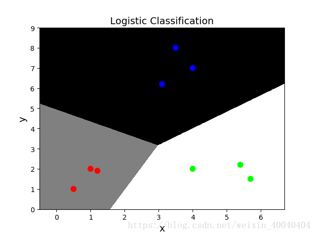
接下来主要介绍如何利用plt.pcolormesh来绘制如下的分类图

plt.pcolormesh的作用在于能够直观表现出分类边界。如果只是单纯的绘制散点图，效果如下：

那么我们就看不出分类的边界。

下面将以鸢尾花数据集为例说明如何使用plt.pcolormesh，该数据集一共包含3类鸢尾花的数据

首先引入必要的库

import numpy as np
import pandas as pd
import matplotlib as mpl
import matplotlib.pyplot as plt
from sklearn.tree import DecisionTreeClassifier

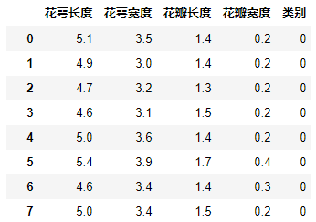
然后读取鸢尾花数据集，并对数据做一定的处理

iris_feature = u'花萼长度', u'花萼宽度', u'花瓣长度', u'花瓣宽度',u'类别'
path = 'iris.data' # 数据文件路径
data = pd.read_csv(path, header=None)
data.columns=iris_feature
data['类别']=pd.Categorical(data['类别']).codes

处理完成后，一共有150组数据，数据长下面这样子

取花萼长度和花瓣长度做为特征，训练决策树模型

x_train = data[['花萼长度','花瓣长度']]
y_train = data['类别']
model = DecisionTreeClassifier(criterion='entropy', min_samples_leaf=3)
model.fit(x_train, y_train)

训练完模型后，现在需要画出分类边界，首先需要在横纵坐标各取500点，一共组成2500个点，然后把这2500个点送进决策树，来算出所属的种类，代码如下：

N, M = 500, 500 # 横纵各采样多少个值
x1_min, x2_min = x_train.min(axis=0)
x1_max, x2_max = x_train.max(axis=0)
t1 = np.linspace(x1_min, x1_max, N)
t2 = np.linspace(x2_min, x2_max, M)
x1, x2 = np.meshgrid(t1, t2) # 生成网格采样点
x_show = np.stack((x1.flat, x2.flat), axis=1) # 测试点
y_predict=model.predict(x_show)

接着就可以绘制出分类图了。由于该数据集中一共有三种鸢尾花，所以绘制图片的时候需要三种颜色

cm_light = mpl.colors.ListedColormap(['#A0FFA0', '#FFA0A0', '#A0A0FF'])
cm_dark = mpl.colors.ListedColormap(['g', 'r', 'b'])

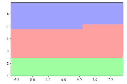
接着使用plt.pcolormesh来绘制分类图

plt.pcolormesh(x1, x2, y_predict.reshape(x1.shape), cmap=cm_light)
plt.show()

plt.pcolormesh()会根据y_predict的结果自动在cmap里选择颜色

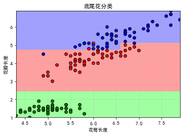
结果如下图

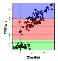
接着再把散点图也画上就大功告成了，结果如下：

完整代码如下

import numpy as np
import pandas as pd
import matplotlib as mpl
import matplotlib.pyplot as plt
from sklearn.tree import DecisionTreeClassifier
iris_feature = u'花萼长度', u'花萼宽度', u'花瓣长度', u'花瓣宽度',u'类别'
path = 'iris.data' # 数据文件路径
data = pd.read_csv(path, header=None)
data.columns=iris_feature
data['类别']=pd.Categorical(data['类别']).codes
x_train = data[['花萼长度','花瓣长度']]
y_train = data['类别']
model = DecisionTreeClassifier(criterion='entropy', min_samples_leaf=3)
model.fit(x_train, y_train)
N, M = 500, 500 # 横纵各采样多少个值
x1_min, x2_min = x_train.min(axis=0)
x1_max, x2_max = x_train.max(axis=0)
t1 = np.linspace(x1_min, x1_max, N)
t2 = np.linspace(x2_min, x2_max, M)
x1, x2 = np.meshgrid(t1, t2) # 生成网格采样点
x_show = np.stack((x1.flat, x2.flat), axis=1) # 测试点
y_predict=model.predict(x_show)
mpl.rcParams['font.sans-serif'] = ['SimHei']
mpl.rcParams['axes.unicode_minus'] = False
cm_light = mpl.colors.ListedColormap(['#A0FFA0', '#FFA0A0', '#A0A0FF'])
cm_dark = mpl.colors.ListedColormap(['g', 'r', 'b'])
plt.xlim(x1_min, x1_max)
plt.ylim(x2_min, x2_max)
plt.pcolormesh(x1, x2, y_predict.reshape(x1.shape), cmap=cm_light)
plt.scatter(x_train['花萼长度'],x_train['花瓣长度'],c=y_train,cmap=cm_dark,marker='o',edgecolors='k')
plt.xlabel('花萼长度')
plt.ylabel('花瓣长度')
plt.title('鸢尾花分类')
plt.grid(True,ls=':')
plt.show()

鹏大大大

关注

3
点赞
踩
22

收藏

觉得还不错? 一键收藏
0
评论
plt.pcolormesh绘制分类图

# -*- coding: utf-8 -*-'''多元分类：逻辑回归分类器并绘制pcolormesh伪彩图sklearn.linear_model.LogisticRegression( solver='liblinear', C=正则强度)'''# pcolormesh(x, y, c=d, cmap='jet') cmap:渐变色映射plt...
复制链接

扫一扫