The extended Kalman Filter

The extended Kalman Filter

Kalman Filter is build according to the assumptions of f linear state transitions and linear measurements with added Gaussian noise,but which are rarely fulfilled in practice.The extended Kalman filter (EKF) overcomes one of these assumptions: the linearity assumption.Here the assumption is that the next state probability and the measurement probabilities are governed by nonlinear functions $g$ and $h$,respectively:

$$\begin{array}{rl}{x}_t& =g\left(u_t,x_{t-1}\right)+{\epsilon }_t\\ z_t& =h\left(x_t\right)+{\delta }_t\end{array}\text{\hspace{1em}(1)}$$

The function $g$ replace the matrixs $A$ and $B$ ,and the $h$ replace the matrix $H$.Unfortunately,the belief is no longer a Gaussian.In fact, performing the belief update exactly is usually impossible.

(写不下去了，切换中文，想想写paper多难。。。)

Linearization Via Taylor Expansion

EKF使用称为 Taylor Expansion 的方法来线性化非线性函数。泰勒展开就是在某点的值和导数构造一个线性approximation。斜率是对某点的偏导数：

$$\begin{array}{r}{g}^{\prime }\left(u_t,x_{t-1}\right):=\frac{\partial g\left(u_t,x_{t-1}\right)}{\partial x_{t-1}}\end{array}$$

其中 $g$ 的值和斜率是取决于 $g$ 的参数的，选取的逻辑就是在线性化的时候最有可能的值，对高斯函数，最有可能的状态就是后验的均值 ${\mu }_{t-1}$ 。换句话说就是 $g$ 在 ${\mu }_{t-1}$ 处 approximate：

$$\begin{array}{rl}g\left(u_t,x_{t-1}\right)& \approx g\left(u_t,{\mu }_{t-1}\right)+\underset{=:G_t}{\underbrace{g^{\prime }\left(u_t,{\mu }_{t-1}\right)}}\left(x_{t-1}-{\mu }_{t-1}\right)\\ & =g\left(u_t,{\mu }_{t-1}\right)+G_t\left(x_{t-1}-{\mu }_{t-1}\right)\end{array}$$

写成概率的表达式可以近似为;

$$\begin{array}{l}p\left(x_t\mid u_t,x_{t-1}\right)\\ \begin{array}{rl}\approx & \det {\left(2\pi R_t\right)}^{-\frac{1}{2}}\exp \{-\frac{1}{2}{\left[x_t-g\left(u_t,{\mu }_{t-1}\right)-G_t\left(x_{t-1}-{\mu }_{t-1}\right)\right]}^T\\ & R_t^{-1}\left[x_t-g\left(u_t,{\mu }_{t-1}\right)-G_t\left(x_{t-1}-{\mu }_{t-1}\right)\right]\}\end{array}\end{array}$$

对测量函数同样线性化，这里的泰勒展开取在 ${\bar{\mu }}_t$ 这附近：

$$\begin{array}{rl}h\left(x_t\right)& \approx h\left({\bar{\mu }}_t\right)+\underset{=:H_t}{\underbrace{h^{\prime }\left({\bar{\mu }}_t\right)}}\left(x_t-{\bar{\mu }}_t\right)\\ & =h\left({\bar{\mu }}_t\right)+H_t\left(x_t-{\bar{\mu }}_t\right)\end{array}$$

写成概率的形式:

$$\begin{array}{rl}p\left(z_t\mid x_t\right)=& \det {\left(2\pi Q_t\right)}^{-\frac{1}{2}}\exp \{-\frac{1}{2}{\left[z_t-h\left({\bar{\mu }}_t\right)-H_t\left(x_t-{\bar{\mu }}_t\right)\right]}^T\\ & Q_t^{-1}\left[z_t-h\left({\bar{\mu }}_t\right)-H_t\left(x_t-{\bar{\mu }}_t\right)\right]\}\end{array}\text{\hspace{1em}(7)}$$

看到这么多字母和数字是不是很头晕？没错我也是，我一开始看也完全不知道这些字母什么意思，你就等等，再把EKF的更新公式放出来，就很清晰了。

The algorithm

我们再把熟悉的KF放上来：

如果对这个类型的KF还是不熟悉，那就再放一个肯定熟悉的：

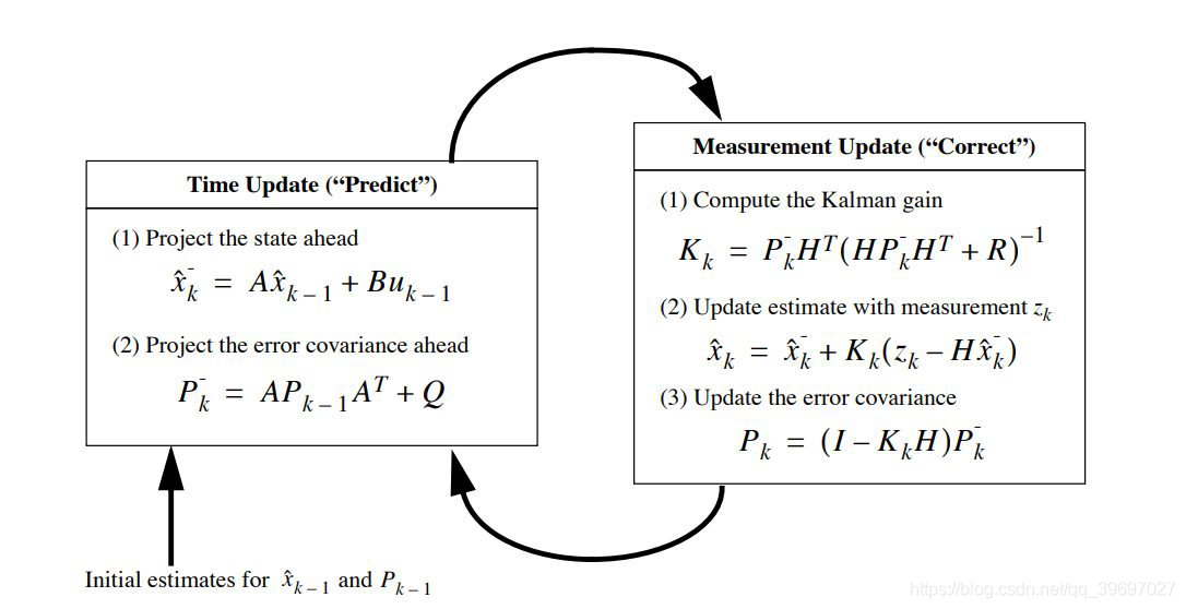
这下对比一下相信已经很熟悉了把，接下来就一个个对应起来理解。第一第二种形式是《Probabilistic Robotics》的，第三种形式是我在这篇intro看到的，第三种看起来更好理解，所以我们就来理一下前两种中字母的关系。

1. ${\bar{\mu }}_t$ equal to ${\hat{x}}_k^{-}$ ,predict state。
2. ${\mu }_t$ equal to ${\hat{x}}_k$ ,represent update the state at $k$ of estimation with measurement。
3. ${\mu }_{t-1}$ equal to ${\hat{x}}_{k-1}$ ,represent the state at $k-1$ of estimation。
4. ${\bar{\Sigma }}_t$ equal to $P_k^{-}$ , a priori estimate error covariance,说人话就是估计的误差协方差矩阵，利用先验的知识，还没有得到观测数据。
5. ${\Sigma }_{t-1}$ equal to $P_{k-1}$ ,a posteriori estimate error covariance,说人话就是利用后验估计误差协方差矩阵，就是利用获得的观测数据更新了误差协方差矩阵。
6. $G_t$ ，$A_t$ and $A$ ,$A$ present a constant transform matrix,but $A_t$ present a dynamic, $G_t$ is a Jacobian matrix,what is Jacobian matrix?Partial derivative of variable matrix.
7. $H_t$ and $H$ and $C_t$ Jacobian $H_t$ corresponds to $C_t$ .

解释完每个变量的意思，就来看看区别：主要的区别是在Predict上:

$$\begin{array}{l}{\bar{\mu }}_t=g\left(u_t,{\mu }_{t-1}\right)\\ {\bar{\Sigma }}_t=G_t{\Sigma }_{t-1}{G}_t^T+R_t\end{array}$$

其中更新predict state不是线性的关系，而是一个非线性的函数 $g$, error covariance 更新需要算协方差矩阵了。这应该就是扩展卡尔曼和卡尔曼的区别了吧。

总结

最后总结就是扩展卡尔曼是一个在某处线性化的过程，而这个线性化的点就在mean of posterior ${\mu }_{t-1}$ ,因为在高斯的图形中，这个mean的点附近是概率最集中的点，这句话应该是精髓吧。然后迭代的过程和卡尔曼滤波是一样的。数学证明有能力有时间再看吧。。。