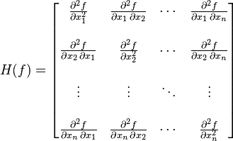
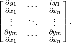
b) 梯度是 Jacobian 矩阵的特例,梯度的 jacobian 矩阵就是 Hesse 矩阵(一阶偏导与二阶偏导的关系)。
3. 优化方法
1) Gradient Descent
Gradient descent 又叫 steepest descent,是利用一阶的梯度信息找到函数局部最优解的一种方法,也是机器学习里面最简单最常用的一种优化方法。Gradient descent 是 line search 方法中的一种,主要迭代公式如下:
其中,是第 k 次迭代我们选择移动的方向,在 steepest descent 中,移动的方向设定为梯度的负方向, 是第 k 次迭代用 line search 方法选择移动的距离,每次移动的距离系数可以相同,也可以不同,有时候我们也叫学习率(learning rate)。在数学上,移动的距离可以通过 line search 令导数为零找到该方向上的最小值,但是在实际编程的过程中,这样计算的代价太大,我们一般可以将它设定位一个常量。考虑一个包含三个变量的函数 ,计算梯度得到 。设定 learning rate = 1,算法代码如下:
# Code from Chapter 11 of Machine Learning: An Algorithmic Perspective# by Stephen Marsland (http://seat.massey.ac.nz/personal/s.r.marsland/MLBook.html)# Gradient Descent using steepest descentfrom numpy import*defJacobian(x):return array([x[0],0.4*x[1],1.2*x[2]])defsteepest(x0):
i =0
iMax =10
x = x0
Delta =1
alpha =1while i<iMax and Delta>10**(-5):
p =-Jacobian(x)
xOld = x
x = x + alpha*p
Delta =sum((x-xOld)**2)print'epoch', i,':'print x,'\n'
i +=1
x0 = array([-2,2,-2])
steepest(x0)
第二步,把 x 看做自变量, 所有带有 x^k 的项看做常量,令一阶导数为 0 ,即可求近似函数的最小值:
即:
第三步,将当前的最小值设定近似函数的最小值(或者乘以步长)。
与 1) 中优化问题相同,牛顿法的代码如下:
# Code from Chapter 11 of Machine Learning: An Algorithmic Perspective# by Stephen Marsland (http://seat.massey.ac.nz/personal/s.r.marsland/MLBook.html)# Gradient Descent using Newton's methodfrom numpy import*defJacobian(x):return array([x[0],0.4*x[1],1.2*x[2]])defHessian(x):return array([[1,0,0],[0,0.4,0],[0,0,1.2]])defNewton(x0):
i =0
iMax =10
x = x0
Delta =1
alpha =1while i<iMax and Delta>10**(-5):
p =-dot(linalg.inv(Hessian(x)),Jacobian(x))
xOld = x
x = x + alpha*p
Delta =sum((x-xOld)**2)
i +=1print x
x0 = array([-2,2,-2])
Newton(x0)
Newton.py
上面例子中由于目标函数是二次凸函数,Taylor 展开等于原函数,所以能一次就求出最优解。
牛顿法主要存在的问题是:
Hesse 矩阵不可逆时无法计算
矩阵的逆计算复杂为 n 的立方,当问题规模比较大时,计算量很大,解决的办法是采用拟牛顿法如 BFGS, L-BFGS, DFP, Broyden's Algorithm 进行近似。
如果初始值离局部极小值太远,Taylor 展开并不能对原函数进行良好的近似
3) Levenberg–Marquardt Algorithm
Levenberg–Marquardt algorithm 能结合以上两种优化方法的优点,并对两者的不足做出改进。与 line search 的方法不同,LMA 属于一种“信赖域法”(trust region),牛顿法实际上也可以看做一种信赖域法,即利用局部信息对函数进行建模近似,求取局部最小值。所谓的信赖域法,就是从初始点开始,先假设一个可以信赖的最大位移 s(牛顿法里面 s 为无穷大),然后在以当前点为中心,以 s 为半径的区域内,通过寻找目标函数的一个近似函数(二次的)的最优点,来求解得到真正的位移。在得到了位移之后,再计算目标函数值,如果其使目标函数值的下降满足了一定条件,那么就说明这个位移是可靠的,则继续按此规则迭代计算下去;如果其不能使目标函数值的下降满足一定的条件,则应减小信赖域的范围,再重新求解。
在很多的资料中,介绍共轭梯度法都举了一个求线性方程组 Ax = b 近似解的例子,实际上就相当于这里所说的
还是用最开始的目标函数 来编写共轭梯度法的优化代码:
# Code from Chapter 11 of Machine Learning: An Algorithmic Perspective# by Stephen Marsland (http://seat.massey.ac.nz/personal/s.r.marsland/MLBook.html)# The conjugate gradients algorithmfrom numpy import*defJacobian(x):#return array([.4*x[0],2*x[1]])return array([x[0],0.4*x[1],1.2*x[2]])defHessian(x):#return array([[.2,0],[0,1]])return array([[1,0,0],[0,0.4,0],[0,0,1.2]])defCG(x0):
i=0
k=0
r =-Jacobian(x0)
p=r
betaTop = dot(r.transpose(),r)
beta0 = betaTop
iMax =3
epsilon =10**(-2)
jMax =5# Restart every nDim iterations
nRestart = shape(x0)[0]
x = x0
while i < iMax and betaTop > epsilon**2*beta0:
j=0
dp = dot(p.transpose(),p)
alpha =(epsilon+1)**2# Newton-Raphson iterationwhile j < jMax and alpha**2* dp > epsilon**2:# Line search
alpha =-dot(Jacobian(x).transpose(),p)/(dot(p.transpose(),dot(Hessian(x),p)))print"N-R",x, alpha, p
x = x + alpha * p
j +=1print x
# Now construct beta
r =-Jacobian(x)print"r: ", r
betaBottom = betaTop
betaTop = dot(r.transpose(),r)
beta = betaTop/betaBottom
print"Beta: ",beta
# Update the estimate
p = r + beta*p
print"p: ",p
print"----"
k +=1if k==nRestart or dot(r.transpose(),p)<=0:
p = r
k =0print"Restarting"
i +=1print x
x0 = array([-2,2,-2])
CG(x0)
参考资料:
[1] Machine Learning: An Algorithmic Perspective, chapter 11 [2] 最优化理论与算法(第2版),陈宝林 [3] wikipedia


 被折叠的 条评论
为什么被折叠?
被折叠的 条评论
为什么被折叠?
 到【灌水乐园】发言


