ML之MIC：利用有无噪音的正余弦函数理解相关性指标的不同(多图绘制Pearson系数、最大信息系数MIC)

ML之MIC：利用有无噪音的正余弦函数理解相关性指标的不同(多图绘制Pearson系数、最大信息系数MIC)

 

 

 

目录

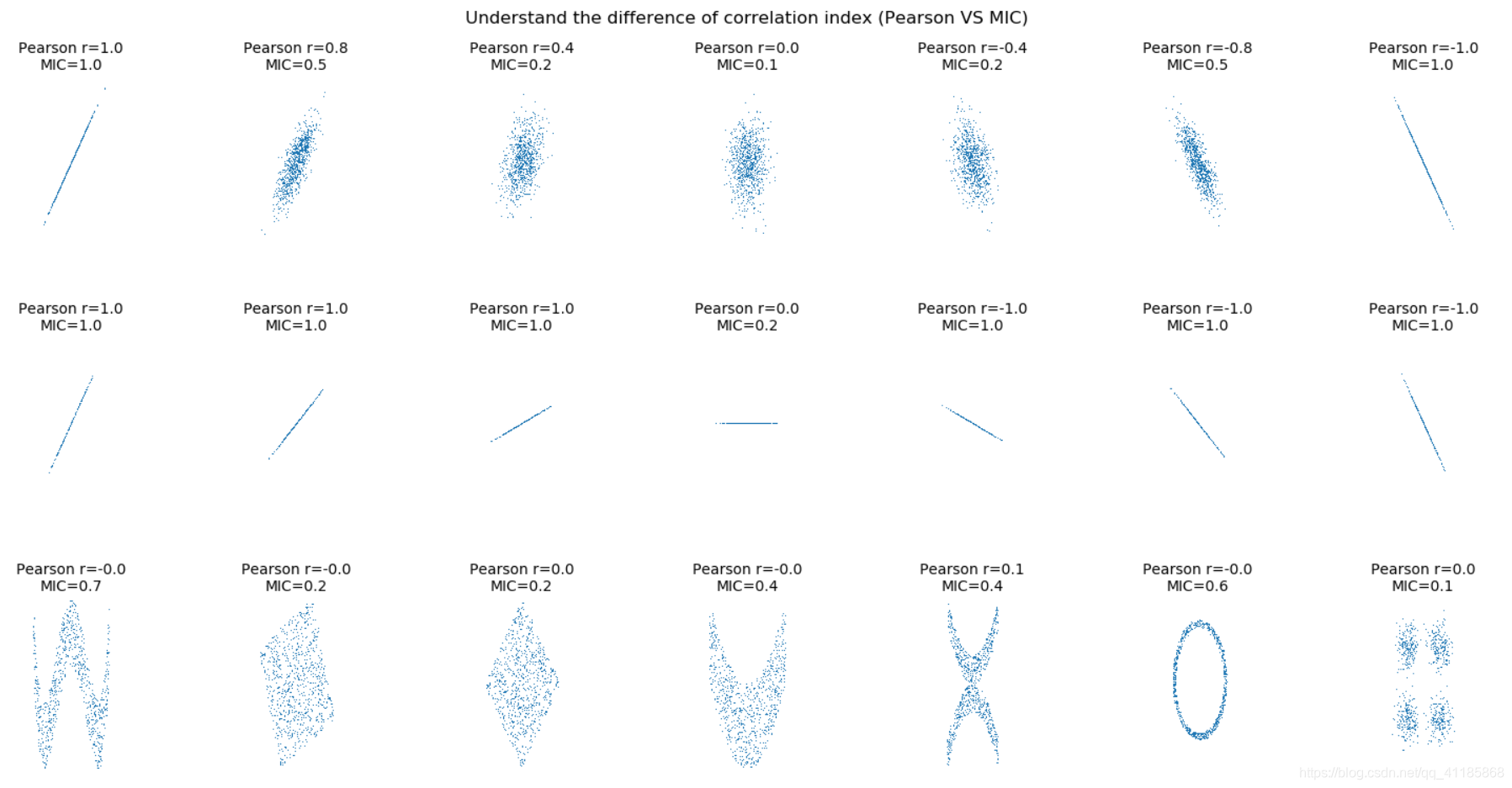
利用有无噪音的正余弦函数理解相关性指标的不同(多图绘制Pearson系数、最大信息系数MIC)

输出结果

实现代码

---

 

 

利用有无噪音的正余弦函数理解相关性指标的不同(多图绘制Pearson系数、最大信息系数MIC)

输出结果

 

 

实现代码

#ML之MIC：利用有无噪音的正余弦函数理解相关性指标的不同(多图绘制Pearson系数、最大信息系数MIC)

import numpy as np
import matplotlib.pyplot as plt
from minepy import MINE
 
 
def mysubplot(x, y, numRows, numCols, plotNum,
              xlim=(-4, 4), ylim=(-4, 4)):
 
    r = np.around(np.corrcoef(x, y)[0, 1], 1)
    mine = MINE(alpha=0.6, c=15)
    mine.compute_score(x, y)
    mic = np.around(mine.mic(), 1)
    ax = plt.subplot(numRows, numCols, plotNum,
                     xlim=xlim, ylim=ylim)
    ax.set_title('Pearson r=%.1f\nMIC=%.1f' % (r, mic),fontsize=10)
    ax.set_frame_on(False)
    ax.axes.get_xaxis().set_visible(False)
    ax.axes.get_yaxis().set_visible(False)
    ax.plot(x, y, ',')
    ax.set_xticks([])
    ax.set_yticks([])
    return ax
 
def rotation(xy, t):
    return np.dot(xy, [[np.cos(t), -np.sin(t)],
                       [np.sin(t), np.cos(t)]])
 
def mvnormal(n=1000):
    cors = [1.0, 0.8, 0.4, 0.0, -0.4, -0.8, -1.0]
    for i, cor in enumerate(cors):
        cov = [[1, cor],[cor, 1]]
        xy = np.random.multivariate_normal([0, 0], cov, n)
        mysubplot(xy[:, 0], xy[:, 1], 3, 7, i+1)
 
def rotnormal(n=1000):
    ts = [0, np.pi/12, np.pi/6, np.pi/4, np.pi/2-np.pi/6,
          np.pi/2-np.pi/12, np.pi/2]
    cov = [[1, 1],[1, 1]]
    xy = np.random.multivariate_normal([0, 0], cov, n)
    for i, t in enumerate(ts):
        xy_r = rotation(xy, t)
        mysubplot(xy_r[:, 0], xy_r[:, 1], 3, 7, i+8)
 
def others(n=1000):
    x = np.random.uniform(-1, 1, n)
    y = 4*(x**2-0.5)**2 + np.random.uniform(-1, 1, n)/3
    mysubplot(x, y, 3, 7, 15, (-1, 1), (-1/3, 1+1/3))
    
    y = np.random.uniform(-1, 1, n)
    xy = np.concatenate((x.reshape(-1, 1), y.reshape(-1, 1)), axis=1)
    xy = rotation(xy, -np.pi/8)
    lim = np.sqrt(2+np.sqrt(2)) / np.sqrt(2)
    mysubplot(xy[:, 0], xy[:, 1], 3, 7, 16, (-lim, lim), (-lim, lim))
 
    xy = rotation(xy, -np.pi/8)
    lim = np.sqrt(2)
    mysubplot(xy[:, 0], xy[:, 1], 3, 7, 17, (-lim, lim), (-lim, lim))
    
    y = 2*x**2 + np.random.uniform(-1, 1, n)
    mysubplot(x, y, 3, 7, 18, (-1, 1), (-1, 3))
    
    y = (x**2 + np.random.uniform(0, 0.5, n)) * \
        np.array([-1, 1])[np.random.random_integers(0, 1, size=n)]
    mysubplot(x, y, 3, 7, 19, (-1.5, 1.5), (-1.5, 1.5))
 
    y = np.cos(x * np.pi) + np.random.uniform(0, 1/8, n)
    x = np.sin(x * np.pi) + np.random.uniform(0, 1/8, n)
    mysubplot(x, y, 3, 7, 20, (-1.5, 1.5), (-1.5, 1.5))
 
    xy1 = np.random.multivariate_normal([3, 3], [[1, 0], [0, 1]], int(n/4))
    xy2 = np.random.multivariate_normal([-3, 3], [[1, 0], [0, 1]], int(n/4))
    xy3 = np.random.multivariate_normal([-3, -3], [[1, 0], [0, 1]], int(n/4))
    xy4 = np.random.multivariate_normal([3, -3], [[1, 0], [0, 1]], int(n/4))
    xy = np.concatenate((xy1, xy2, xy3, xy4), axis=0)
    mysubplot(xy[:, 0], xy[:, 1], 3, 7, 21, (-7, 7), (-7, 7))
 
plt.figure(facecolor='white')
mvnormal(n=800)
rotnormal(n=200)
others(n=800)
plt.tight_layout()

plt.suptitle('Understand the difference of correlation index (Pearson VS MIC)')
plt.show()