R语言空间数据分析学习笔记6——空间点分布特征

这次对空间点特征进行学习：

library(pacman)
p_load(spatstat,sp,rgeos,maptools,GISTools,tmap,sf,
       geojson,geojsonio,tmaptools,tidyverse,raster,fpc,dbscan,ggplot2)

LondonBoroughs <-st_read(
  "G:/Rdata/boundaries_london/ESRI/London_Borough_Excluding_MHW.shp"
)

#把特定的区域提取出来，并转化为特定的坐标系
BoroughMap <- LondonBoroughs %>%
  dplyr::filter(str_detect(GSS_CODE,"^E09")) %>%
  st_transform(.,27700)
tmap_mode("view")
qtm(BoroughMap)

#把建筑物矢量点加进来
BluePlaques <- st_read("https://s3.eu-west-2.amazonaws.com/openplaques/open-plaques-london-2018-04-08.geojson") %>%
  st_transform(.,27700)
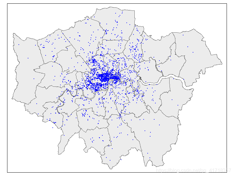
tmap_mode("plot")
tm_shape(BoroughMap)+
  tm_polygons(col=NA, alpha = 0.5)+
  tm_shape(BluePlaques)+
  tm_dots(col="blue")

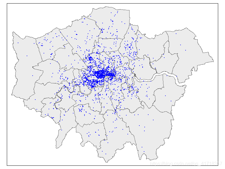
#去重(distinct)+提取伦敦范围内的名人建筑,从上图可以看出有部分名人建筑在伦敦范围外了
BluePlaques1 <- distinct(BluePlaques)  #从2812-2711
BluePlaques2 <- BluePlaques1[BoroughMap,] #从2711-2697
tm_shape(BoroughMap)+
  tm_polygons(col=NA,alpha = 0.5)+
  tm_shape(BluePlaques2)+
  tm_dots(col="blue")

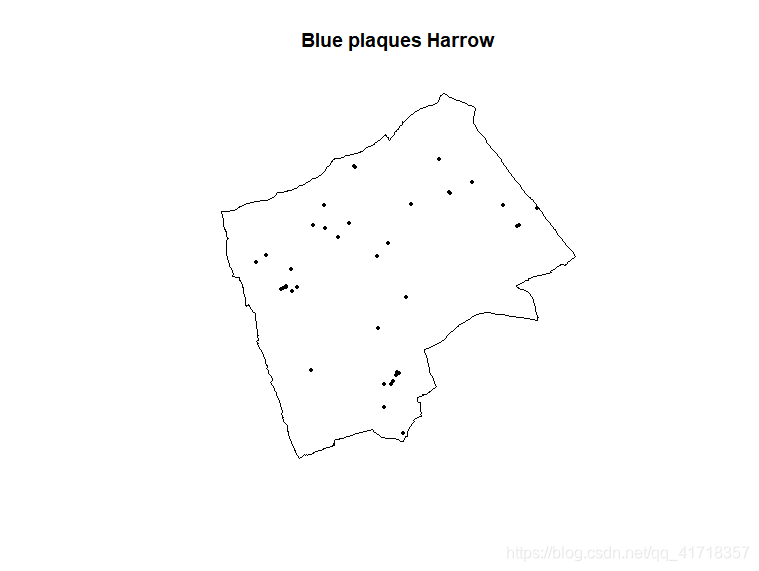
#让我们提取其中一块区域，并进行可视化
Harrow <- BoroughMap %>%
  filter(.,NAME=="Harrow")
BluePlaques3 <- BluePlaques2[Harrow,] #39个名人建筑


tmap_mode("view")
tm_shape(Harrow)+
  tm_polygons(col=NA,alpha = 0.5)+
  tm_shape(BluePlaques3)+
  tm_dots("blue")

#下面进行空间点过程模拟，由于这需要用到spatsta包，必须要让数据格式符合个包函数能接受的形式，转化如下：
#now set a window  as the borough boundary
window <- as.owin(Harrow)
#create a ppp object
BluePlaques4 <- BluePlaques3 %>%
  as(., 'Spatial')
BluePlaques4.ppp<-ppp(x=BluePlaques4@coords[,1],
                      y=BluePlaques4@coords[,2],
                      window = window)
BluePlaques4.ppp %>%
  plot(.,pch=16,cex=0.5,
       main="Blue plaques Harrow")
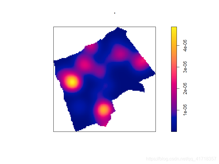
#上述代码可以看到，ppp对象的的建立最关键的，其中X和Y接受的是经纬度信息，然后需要用as.owin
#来转化其底层的地理信息，然后我们可以根据这些信息，来观测点过程模型生成的图
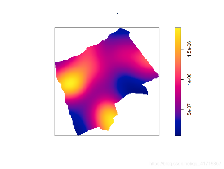
BluePlaques4.ppp %>%
  density(., sigma=500)%>%
  plot()

#这里，sigma控制的是辐射半径，设置大一点的话，则这些点的辐射范围会更大。
BluePlaques4.ppp %>%
  density(.,sigma=1000)%>%
  plot()

#我们想知道这些点在空间中是不是随机分布的，可以使用样方分析
teststats <- quadrat.test(BluePlaques4.ppp,nx=6,ny=6)
teststats
# Chi-squared test of CSR using quadrat counts
# 
# data:  BluePlaques4.ppp
# X2 = 37.969, df = 28, p-value = 0.198
# alternative hypothesis: two.sided
#P值大于0.05,因此不能拒绝它是随机分布(泊松分布)的假设，红色部分分别是模拟值，观测值和Pearson残差。

plot(BluePlaques4.ppp,pch=16,cex=0.5,main="Blue Plaques in Harrow")
plot(teststats,add=T,col="red")

#另一种方法是K检验，这种方法能得到另一种解释强的结论。
K <- BluePlaques4.ppp %>%
  Kest(., correction = "border")%>%
  plot()

#这个结果表示，在1300m一下的尺度上，点呈现聚集分布，而在1600-2100m之间，点呈现规则分布，
#如果想要做点与点之间的聚类，可以使用DBSCAN算法,实现代码如下
#first extract the points from the spatial points data frame 
BluePlaquesSubPoints <- BluePlaques4 %>%
  coordinates(.)%>%
  as.data.frame()

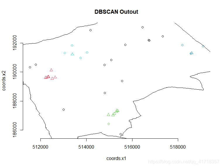
#now run the dbscan analysis
db <- BluePlaquesSubPoints %>%
  fpc::dbscan(.,eps=700, MinPts = 4)#esp控制空间聚类的尺度，MinPts控制最少聚类点数量
#now plot the results
plot(db,BluePlaquesSubPoints,main="DBSCAN Outout",frame = F)
plot(BoroughMap$geometry,add=T)
 
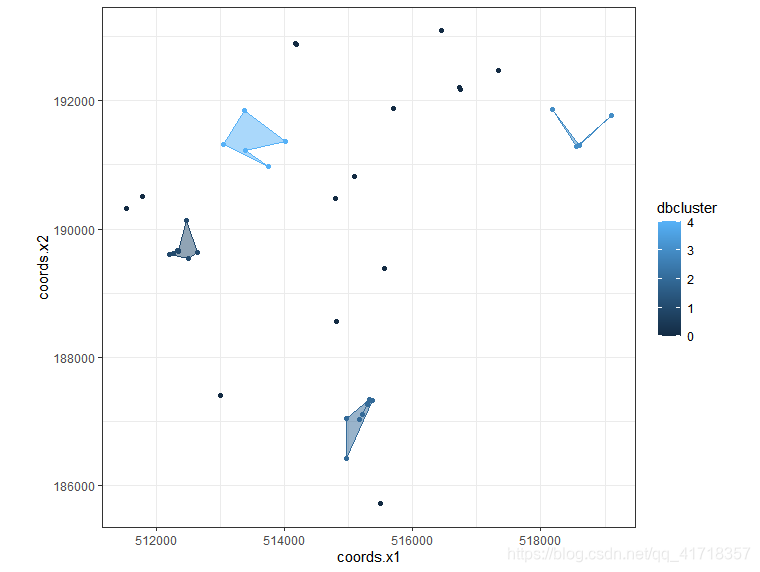
#使用ggplot2进行可视化，可以这样实现
BluePlaquesSubPoints <- BluePlaquesSubPoints%>%
  mutate(dbcluster=db$cluster)
chulls <- BluePlaquesSubPoints %>%
  group_by(dbcluster) %>%
  dplyr::mutate(hull=1:n(),
                hull=factor(hull,chull(coords.x1,coords.x2)))%>%
  arrange(hull)%>%
  filter(dbcluster >=1)


dbplot <- ggplot(data=BluePlaquesSubPoints,
                 aes(coords.x1, coords.x2, colour=dbcluster, fill=dbcluster))
dbplot
#add the points in
dbplot <- dbplot+geom_point()
dbplot
#now convex the hulls
dbplot <- dbplot + geom_polygon(data=chulls,
                               aes(coords.x1,coords.x2,group=dbcluster),
                               alpha=0.5)
dbplot
#now plot,setting the coordinates to scale correctly and as a black and write plot
#(just for the hell of it)...
bdplot + theme_bw()+coord_equal()