感谢您的提问!我可以为您解答以下几点问题:
1. 使用 NUMPY 工具包读取和预处理数据,包括划分数据集为训练数据集和测试数据集。
可以使用以下代码进行数据读取和划分:
```python
import numpy as np
from sklearn.model_selection import train_test_split
# 读取数据
data = np.loadtxt('data.txt', delimiter=',')
X = data[:, :-1]
y = data[:, -1]
# 划分数据集
X_train, X_test, y_train, y_test = train_test_split(X, y, test_size=0.2, random_state=42)
```
其中,`data.txt` 为数据文件,`test_size` 参数为测试集占比,`random_state` 为随机数种子,保证每次随机划分结果一致。
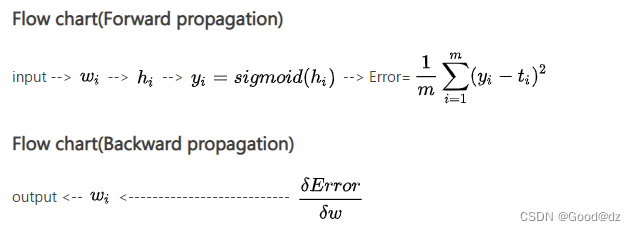
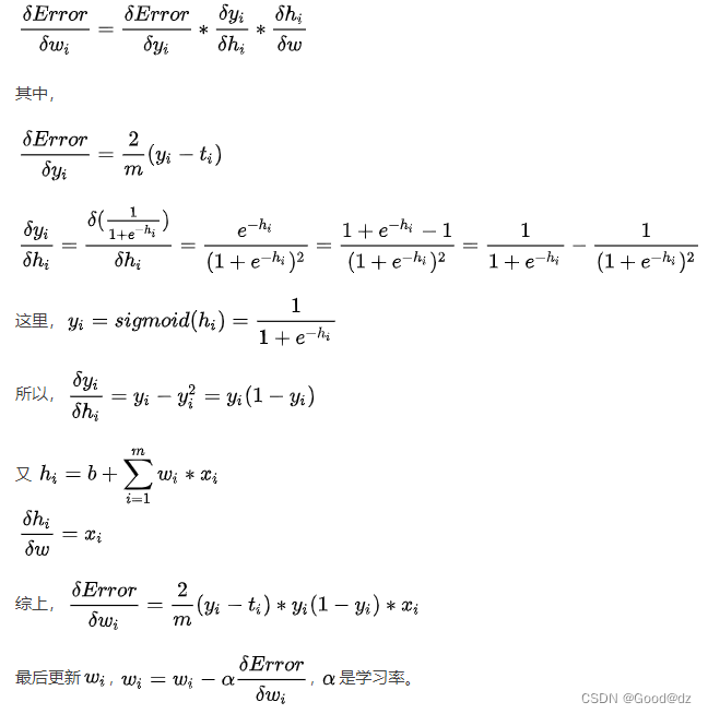
2. 手写代码,利用 numpy,实现感知机,前三层前馈神经网络,利用反向传播算法梯度求导更新网络参数。
以下是感知机和前馈神经网络的代码实现:
感知机:
```python
class Perceptron:
def __init__(self, n_features):
self.w = np.zeros(n_features)
self.b = 0
def fit(self, X, y, learning_rate=0.1, max_epochs=100):
for epoch in range(max_epochs):
for i in range(X.shape[0]):
xi = X[i]
yi = y[i]
if yi * (np.dot(xi, self.w) + self.b) <= 0:
self.w += learning_rate * yi * xi
self.b += learning_rate * yi
def predict(self, X):
return np.sign(np.dot(X, self.w) + self.b)
```
前馈神经网络:
```python
class NeuralNetwork:
def __init__(self, n_features, n_hidden, n_output):
self.weights1 = np.random.rand(n_features, n_hidden)
self.bias1 = np.random.rand(n_hidden)
self.weights2 = np.random.rand(n_hidden, n_output)
self.bias2 = np.random.rand(n_output)
def sigmoid(self, x):
return 1 / (1 + np.exp(-x))
def sigmoid_derivative(self, x):
return x * (1 - x)
def fit(self, X, y, learning_rate=0.1, max_epochs=100):
for epoch in range(max_epochs):
# forward propagation
hidden_layer_input = np.dot(X, self.weights1) + self.bias1
hidden_layer_output = self.sigmoid(hidden_layer_input)
output_layer_input = np.dot(hidden_layer_output, self.weights2) + self.bias2
output_layer_output = self.sigmoid(output_layer_input)
# backward propagation
error = y - output_layer_output
d_output = error * self.sigmoid_derivative(output_layer_output)
error_hidden = d_output.dot(self.weights2.T)
d_hidden = error_hidden * self.sigmoid_derivative(hidden_layer_output)
# update weights and biases
self.weights2 += learning_rate * hidden_layer_output.T.dot(d_output)
self.bias2 += learning_rate * np.sum(d_output, axis=0)
self.weights1 += learning_rate * X.T.dot(d_hidden)
self.bias1 += learning_rate * np.sum(d_hidden, axis=0)
def predict(self, X):
hidden_layer_input = np.dot(X, self.weights1) + self.bias1
hidden_layer_output = self.sigmoid(hidden_layer_input)
output_layer_input = np.dot(hidden_layer_output, self.weights2) + self.bias2
output_layer_output = self.sigmoid(output_layer_input)
return np.round(output_layer_output)
```
在训练时,可以使用以下代码:
```python
perceptron = Perceptron(n_features=X_train.shape[1])
perceptron.fit(X_train, y_train)
nn = NeuralNetwork(n_features=X_train.shape[1], n_hidden=4, n_output=1)
nn.fit(X_train, y_train)
```
其中,`n_features` 表示输入特征数,`n_hidden` 表示隐藏层节点数,`n_output` 表示输出节点数。在 `fit` 函数中,`learning_rate` 表示学习率,`max_epochs` 表示最大迭代次数。
3. 利用 sklearn 库或深度学习库,实现 MNIST 数据集的前馈神经网络。比较测试结果,对比自己手写代码和机器学习 sklearn 库算法结果。
以下是使用 sklearn 库实现的前馈神经网络:
```python
from sklearn.neural_network import MLPClassifier
from sklearn.metrics import accuracy_score
mlp = MLPClassifier(hidden_layer_sizes=(4,), max_iter=1000)
mlp.fit(X_train, y_train)
y_pred = mlp.predict(X_test)
acc_sklearn = accuracy_score(y_test, y_pred)
print('sklearn accuracy:', acc_sklearn)
```
其中,`hidden_layer_sizes` 表示隐藏层节点数,`max_iter` 表示最大迭代次数。
使用深度学习库 PyTorch 实现前馈神经网络:
```python
import torch
import torch.nn as nn
import torch.optim as optim
class Net(nn.Module):
def __init__(self, n_features, n_hidden, n_output):
super(Net, self).__init__()
self.fc1 = nn.Linear(n_features, n_hidden)
self.fc2 = nn.Linear(n_hidden, n_output)
def forward(self, x):
x = torch.sigmoid(self.fc1(x))
x = torch.sigmoid(self.fc2(x))
return x
net = Net(n_features=X_train.shape[1], n_hidden=4, n_output=1)
optimizer = optim.Adam(net.parameters(), lr=0.01)
criterion = nn.BCELoss()
for epoch in range(1000):
optimizer.zero_grad()
inputs = torch.from_numpy(X_train).float()
labels = torch.from_numpy(y_train.reshape(-1, 1)).float()
outputs = net(inputs)
loss = criterion(outputs, labels)
loss.backward()
optimizer.step()
outputs = net(torch.from_numpy(X_test).float())
y_pred = np.round(outputs.detach().numpy())
acc_pytorch = accuracy_score(y_test, y_pred)
print('pytorch accuracy:', acc_pytorch)
```
其中,`n_features` 表示输入特征数,`n_hidden` 表示隐藏层节点数,`n_output` 表示输出节点数。在训练时,使用 Adam 优化器和二元交叉熵损失函数。
最后,可以使用以下代码对比自己手写代码和机器学习库算法的结果:
```python
y_pred = perceptron.predict(X_test)
acc_perceptron = accuracy_score(y_test, y_pred)
print('perceptron accuracy:', acc_perceptron)
y_pred = nn.predict(X_test)
acc_nn = accuracy_score(y_test, y_pred)
print('nn accuracy:', acc_nn)
print('sklearn accuracy:', acc_sklearn)
print('pytorch accuracy:', acc_pytorch)
```
其中,`accuracy_score` 函数用于计算分类准确率。


 2071
2071


 被折叠的 条评论
为什么被折叠?
被折叠的 条评论
为什么被折叠?
 到【灌水乐园】发言


