


数字图像处理——局部直方图均衡化【像素级别处理】(python)
局部直方图处理是弄一个略大于图片的矩阵,超过图片的部分用0来代替像素值,在这个局部进行直方图均衡化。
输入:

import cv2
import numpy as np
import matplotlib.pyplot as plt
import datetime
# 局部直方图处理 3.3.3节
# 使用3*3的领域处理
img = cv2.imread('Fig0326.tif') # 局部信息图片
H = img.shape[0]
W = img.shape[1]
hr = np.zeros(256) # 原始直方图信息
pr = np.zeros(256) # 原始图片的概率
rtos = np.zeros(256) # r->s的映射
# 计算原始图片的像素分布图和概率密度函数
for row in range(H):
for col in range(W):
hr[img[row, col]] += 1
for i in range(256):
pr[i] = hr[i] / (H * W)
for i in range(256): # i=[0,255]
for j in range(i + 1): # j=[0,i]
rtos[i] += pr[j]
rtos[i] = round(rtos[i] * 255) # 四舍五入取整
hisImg = np.zeros((H, W, 3), np.uint8) # 建立直方图均衡变换之后的图片
for row in range(H):
for col in range(W):
hisImg[row, col] = rtos[img[row, col]]
# 局部直方图变换,使用3*3的邻域统计直方图
localsize = 3 # 邻域的尺寸为3*3,这个邻域值最好为奇数
tempImg = np.zeros((H + localsize - 1, W + localsize - 1, 3), np.uint8) # 创建一个边界大一半领域像素的值,以便统计边缘像素
localHistImg = np.zeros((H, W, 3), np.uint8) # 存储新图
for row in range(H):
for col in range(W):
tempImg[row + (localsize - 1) // 2, col + (localsize - 1) // 2] = img[row, col]
# f = open('out.txt', 'w')
starttime = datetime.datetime.now()
for row in range((localsize - 1) // 2, H + (localsize - 1) // 2):
for col in range((localsize - 1) // 2, W + (localsize - 1) // 2): # 外层大循环
# 每行统计新加入的点和删除的点是否具有相同的灰度值,这里localsize是3,所以用row,row-1,row+1三行
# 只要比较0通道的值就行,对于灰度图来说,三个通道的值相同
if row <= (localsize - 1) // 2 or col <= (localsize - 1) // 2 \
or row > H - 1 or col > W - 1 \
or tempImg[row, col - 2, 0] != tempImg[row, col + 2, 0] \
or tempImg[row - 1, col - 2, 0] != tempImg[row - 1, col + 2, 0] \
or tempImg[row + 1, col - 2, 0] != tempImg[row + 1, col + 2, 0]:
# 每一行一列重新计算概率分布
for i in range(256):
pr[i] = 0
rtos[i] = 0
for i in range(localsize):
for j in range(localsize):
pr[tempImg[row + (i - (localsize - 1) // 2), col + (j - (localsize - 1) // 2)]] += 1
for i in range(256):
for j in range(i + 1):
rtos[i] += pr[j]
rtos[i] = round(rtos[i] * 255 / (localsize * localsize))
localHistImg[row - (localsize - 1) // 2, col - (localsize - 1) // 2] = rtos[tempImg[row, col]]
# f.close()
endtime = datetime.datetime.now()
print(endtime - starttime)
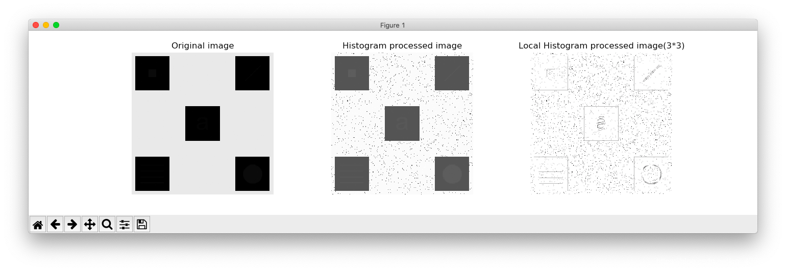
# 原图
plt.subplot(1, 3, 1)
plt.axis('off')
plt.title('Original image')
plt.imshow(img)
# 直方图均衡后的图
plt.subplot(1, 3, 2)
plt.axis('off')
plt.title('Histogram processed image')
plt.imshow(hisImg)
# 直方图均衡后的图
plt.subplot(1, 3, 3)
plt.axis('off')
plt.title('Local Histogram processed image(3*3)')
plt.imshow(localHistImg)
plt.show()
输出:


 7653
7653


 被折叠的 条评论
为什么被折叠?
被折叠的 条评论
为什么被折叠?
 到【灌水乐园】发言


