


In [139]:
import matplotlib.pyplot as plt
%matplotlib notebook
import seaborn as sns
sns.set(style='whitegrid', context='notebook')
sns.reset_orig()

import pandas as pd
import numpy as np
import scipy as sp
import scipy.io
In [111]:
df = pd.DataFrame(data={'y': [1, 2, 3],
                       'score': [93.5, 89.4, 90.3],
                       'name': ['Dirac', 'Pauli', 'Bohr'],
                       'birthday': ['1902-08-08', '1900-04-25', '1895-10-07']})
print(type(df))
print(df.dtypes)
df
Out[111]:
In [112]:
df.to_csv("./test.csv")
In [113]:
df = pd.read_csv('./test.csv')
df
Out[113]:
In [114]:
items = pd.Series(data=[93.5, 89.4, 90.3], name='score')
print(type(items))
items
Out[114]:
In [115]:
items2 = pd.Series(data=['1902-08-08', '1900-04-25'], name='birthday')
print('')
print(items2)
print('')
print('按列合并到一起:')
print(pd.concat(objs=[items, items2], axis=0))
print('')
print('按行合并到一起:')
print(pd.concat(objs=[items, items2], axis=1))
In [116]:
pd.to_datetime(arg=df.birthday, format='%Y-%m-%d')
Out[116]:
In [41]:
df_new = pd.DataFrame(data=list(zip(['Dirac', 'Pauli', 'Bohr', 'Einstein'],
                                    [True, False, True, True])),
                      columns=['name', 'friendly'])

df_merge = pd.merge(left=df, right=df_new, on='name', how='outer')
df_merge
Out[41]:
In [117]:
pd.date_range(start=df.birthday[2], end=df.birthday[0],
              freq='M')
Out[117]:
In [119]:
df = pd.read_table(filepath_or_buffer='test.csv')
df
Out[119]:
In [128]:
import pandas.util.testing as tm
tm.np.random.choice(['red','green'], 10)
Out[128]:
In [121]:
test_list = [[None, 1, 2, 3, 4], [None, 1, None, 3, None]]
print(pd.isnull(test_list))

pd.isnull(df_merge)
Out[121]:
In [46]:
np.array(object=[[1, 9, 9, 1], [2, 0, 1, 6]], dtype=np.float32)
Out[46]:
In [47]:
np.zeros(shape=(2, 4), dtype=int)
Out[47]:
In [48]:
np.arange(start=1.5, stop=8.5, step=0.7, dtype=float)
Out[48]:
In [49]:
np.sqrt([16, 9, 4])
Out[49]:
In [50]:
np.ones(shape=(2, 3, 1), dtype=np.unicode)
Out[50]:
In [51]:
vals = np.arange(0, 12, 1).reshape((3, 4))
print(vals)
print('')
print('sum entire array =', np.sum(vals))
print('sum along columns =', np.sum(vals, axis=0))
print('sum along rows =', np.sum(vals, axis=1))
In [52]:
vals = np.array([1, 2, 3, 4]*3).reshape((3, 4))
print(vals)
print('')
print('mean entire array =', np.mean(vals))
print('mean along columns =', np.mean(vals, axis=0))
print('mean along rows =', np.mean(vals, axis=1))
In [53]:
np.linspace(0, 19.3, 6)
Out[53]:
In [54]:
vals = np.array([9, 2, 3, 5])
print(type(vals))
print(vals)
a = np.asarray(vals)
a += 1
print(vals) # vals changes because it was not copied when assigning 'a'
In [129]:
# 得到标准差,忽略NA
vals = [0.0, np.nan, 8.3, 2.4, np.nan, 3.2]
sp.nanstd(vals)
Out[129]:
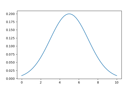
In [140]:
# 正态分布
x = np.linspace(0,10,50)
# 画高斯曲线
plt.plot(x, sp.stats.norm.pdf(x=x, loc=5, scale=2))
# 高斯随机样本
sp.stats.norm.rvs(loc=5, scale=2, size=4)
plt.show()
In [59]:
vals = np.array([[0, 3.4, 2], [0, 9.9, 0], [0, 0, -5.4]])
print(vals)
print('')
a = sp.sparse.csr_matrix(vals)
print(type(a))
print('non-zero entries =', a.data) # 稀疏矩阵中元素的个数
print('diagonal entries =',a.diagonal())# 对角数据
print('upper triangular =\n',sp.sparse.triu(a))
In [141]:
# 求函数的根

f = lambda x: x**2 - 3*x + 2 # = (x-1)*(x-2)
print(f)
roots = (sp.optimize.brentq(f=f, a=0, b=1.5),
         sp.optimize.brentq(f=f, a=1.5, b=5))
print('First root =', roots[0])
print('Second root =', roots[1])
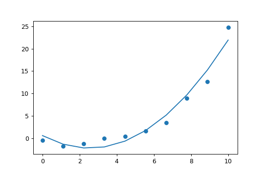
In [143]:
# 最小二乘法参数优化

x = np.linspace(0, 10, 10)
y = np.array([-0.5, -1.8, -1.3, -0.1, 0.4,
              1.6, 3.5, 8.9, 12.6, 24.8])

# 二次函数形式拟合
f = lambda beta, x:  beta[0] + beta[1]*x + beta[2]*x**2

# f和实际值之间的差异
error_function = lambda beta, x, y: f(beta, x) - y

beta_0 = (0.0, 0.0, 0.0)

beta, _ = sp.optimize.leastsq(func=error_function, x0=beta_0, args=(x, y))
print('optimal parameters =', beta)
plt.scatter(x, y);
plt.plot(x, [f(beta, xx) for xx in x])
plt.show()
In [62]:
# 将数组转换成matlab数据

# 初始化数组
np.set_printoptions(precision=1)
matrix = np.random.random(size=(8, 6))
print(matrix)

# 创建行字典
data_dict = {'row'+str(r_id): row for r_id, row in
             zip(range(len(matrix)), matrix)}
# 将每行变量,写入matlab文件
scipy.io.savemat('random_array.mat', mdict=data_dict, oned_as='row')

# 读取刚保存的数据
loaded_data_dict = scipy.io.loadmat('random_array.mat')
loaded_data_dict
Out[62]:
In [63]:
matrix = np.array([[4.3, 8.9],[2.2, 3.4]])
print(matrix)
print('')

# 求范数
norm = sp.linalg.norm(matrix)
print('norm =', norm)
# Alternate method
print(norm == np.square([v for row in matrix for v in row]).sum()**(0.5))
print('')

# 求特征值和特征向量
eigvals, eigvecs = sp.linalg.eig(matrix)
print('eigenvalues =', eigvals)
print('eigenvectors =\n', eigvecs)
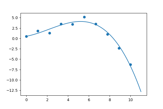
In [144]:
# 散点拟合

x = np.linspace(0, 10, 10)
xs = np.linspace(0, 11, 50)
y = np.array([0.5, 1.8, 1.3, 3.5, 3.4,
              5.2, 3.5, 1.0, -2.3, -6.3])
spline = sp.interpolate.UnivariateSpline(x, y)
plt.scatter(x, y);
plt.plot(xs, spline(xs))
plt.show()
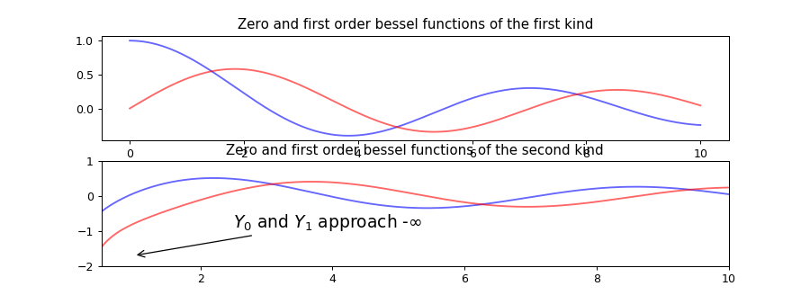
In [145]:
x = np.linspace(0,10,500)
fix, ax = plt.subplots(2)

ax[0].set_title('Zero and first order bessel functions of the first kind')
ax[0].plot(x, sp.special.j0(x), c='blue', alpha=0.6)
ax[0].plot(x, sp.special.j1(x), c='red', alpha=0.6)

ax[1].set_title('Zero and first order bessel functions of the second kind')
ax[1].plot(x, sp.special.y0(x), c='blue', alpha=0.6)
ax[1].plot(x, sp.special.y1(x), c='red', alpha=0.6)
ax[1].set_ylim(-2,1); ax[1].set_xlim(0.5,10)
ax[1].annotate('$Y_0$ and $Y_1$ approach -$\infty$', xy=(1,-1.7), xytext=(2.5, -0.9),
               arrowprops=dict(arrowstyle='->', lw=1), fontsize=15)

plt.show()
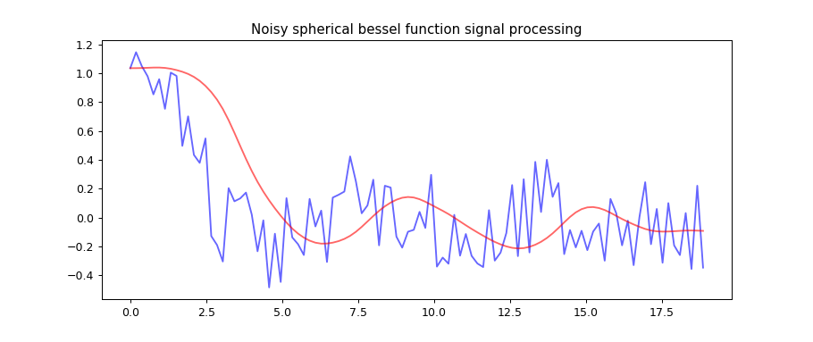
In [146]:
# A modified example posted in the docs:
# http://docs.scipy.org/doc/scipy/reference/generated/scipy.signal.lfilter.html#scipy.signal.lfilter

import scipy.signal
np.random.seed(0)

x = np.linspace(0,6*np.pi,100)
y = [sp.special.sph_jn(n=3, z=xi)[0][0] for xi in x]
y = [yi + (np.random.random()-0.5)*0.7 for yi in y]
# y = np.sin(x)

# 得到一个3阶低通巴特沃斯滤波器参数
b, a = sp.signal.butter(3, 0.08)

# Initialize filter
zi = sp.signal.lfilter_zi(b, a)

# Apply filter
y_smooth, _ = sp.signal.lfilter(b, a, y, zi=zi*y[0])

plt.plot(x, y, c='blue', alpha=0.6)
plt.plot(x, y_smooth, c='red', alpha=0.6)
plt.title('Noisy spherical bessel function signal processing')
plt.savefig('noisy_signal_fit.png', bbox_inches='tight')
plt.show()
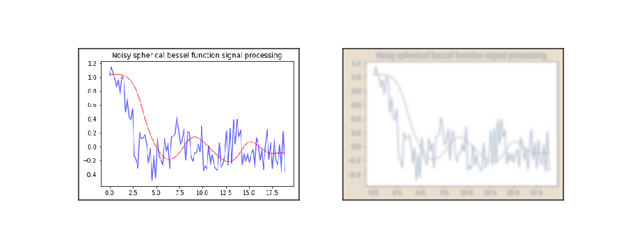
In [148]:
# 模糊图像

# 导入图像
figure = plt.imread('noisy_signal_fit.png')

# 模糊图像
figure_blur = sp.ndimage.filters.gaussian_filter(figure, sigma=2)# sigma值越大。越模糊

# 画图
pics = [figure, figure_blur]
sns.set_style('white')
fig, axes = plt.subplots(1, 2, figsize=(10, 4))
for pic, ax in zip(pics, axes):
    ax.imshow(pic); ax.set_xticks([]); ax.set_yticks([])
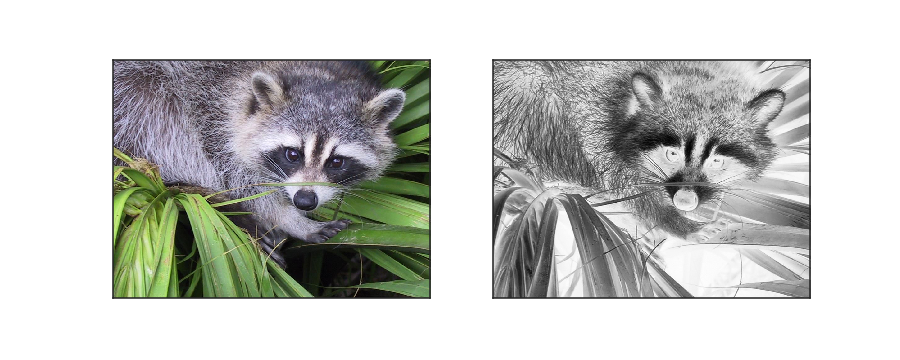
In [149]:
# 获得浣熊脸

# 获取浣熊
pics = sp.misc.face(), sp.misc.face(gray=True)

# 画出来
fig, axes = plt.subplots(1, 2, figsize=(10, 4))
for pic, ax in zip(pics, axes):
    ax.imshow(pic); ax.set_xticks([]); ax.set_yticks([])
plt.show()


 2254
2254


 被折叠的 条评论
为什么被折叠?
被折叠的 条评论
为什么被折叠?
 到【灌水乐园】发言


