Unet项目解析(4): ./src/RetinaNN_predict.py

项目GitHub主页：https://github.com/orobix/retina-unet

参考论文：Retina blood vessel segmentation with a convolution neural network (U-net) Retina blood vessel segmentation with a convolution neural network (U-net)

1.导入相关模块

#Python
import numpy as np
import configparser
from matplotlib import pyplot as plt
#Keras
from keras.models import model_from_json

导入sklearn模块，关于sklearn模块的详细说明可以参考fuqiuai的博客，也可以参考官网的使用说明。

sklearn.metric提供了一些函数，用来计算真实值与预测值之间的预测误差；这里用的评价标准主要集中如下几个方面：

#scikit learn
from sklearn.metrics import roc_curve
from sklearn.metrics import roc_auc_score
from sklearn.metrics import confusion_matrix
from sklearn.metrics import precision_recall_curve
from sklearn.metrics import jaccard_similarity_score
from sklearn.metrics import f1_score

导入依赖的处理脚本文件。

import sys
sys.path.insert(0, '/home/shenziehng/anaconda/SpyderProject/Retina_NN/lib/')
# help_functions.py
from help_functions import *
# extract_patches.py
from extract_patches import recompone
from extract_patches import recompone_overlap
from extract_patches import paint_border
from extract_patches import kill_border
from extract_patches import pred_only_FOV
from extract_patches import get_data_testing
from extract_patches import get_data_testing_overlap
# pre_processing.py
from pre_processing import my_PreProc

2. 加载配置文件，解析参数

config = configparser.RawConfigParser()
config.read('/home/shenziheng/SpyderProject/Retina_NN/configuration.txt')
path_data = config.get('data paths', 'path_local') #数据路径
DRIVE_test_imgs_original = path_data + config.get('data paths', 'test_imgs_original') #测试集图像封装文件
test_imgs_orig = load_hdf5(DRIVE_test_imgs_original) #测试集图像
full_img_height = test_imgs_orig.shape[2]
full_img_width = test_imgs_orig.shape[3]

DRIVE_test_border_masks = path_data + config.get('data paths', 'test_border_masks') #测试集掩膜封装文件
test_border_masks = load_hdf5(DRIVE_test_border_masks)
# 图像块的维度
patch_height = int(config.get('data attributes', 'patch_height'))
patch_width = int(config.get('data attributes', 'patch_width'))
# 图像分块的跳跃步长
stride_height = int(config.get('testing settings', 'stride_height'))
stride_width = int(config.get('testing settings', 'stride_width'))
assert (stride_height < patch_height and stride_width < patch_width)

name_experiment = config.get('experiment name', 'name')
path_experiment = './' +name_experiment +'/'

Imgs_to_test = int(config.get('testing settings', 'full_images_to_test')) # 20张图像全部进行预测

N_visual = int(config.get('testing settings', 'N_group_visual')) #1

average_mode = config.getboolean('testing settings', 'average_mode') # average=True


#ground truth
gtruth= path_data + config.get('data paths', 'test_groundTruth') #测试集金标准封装文件
img_truth= load_hdf5(gtruth)

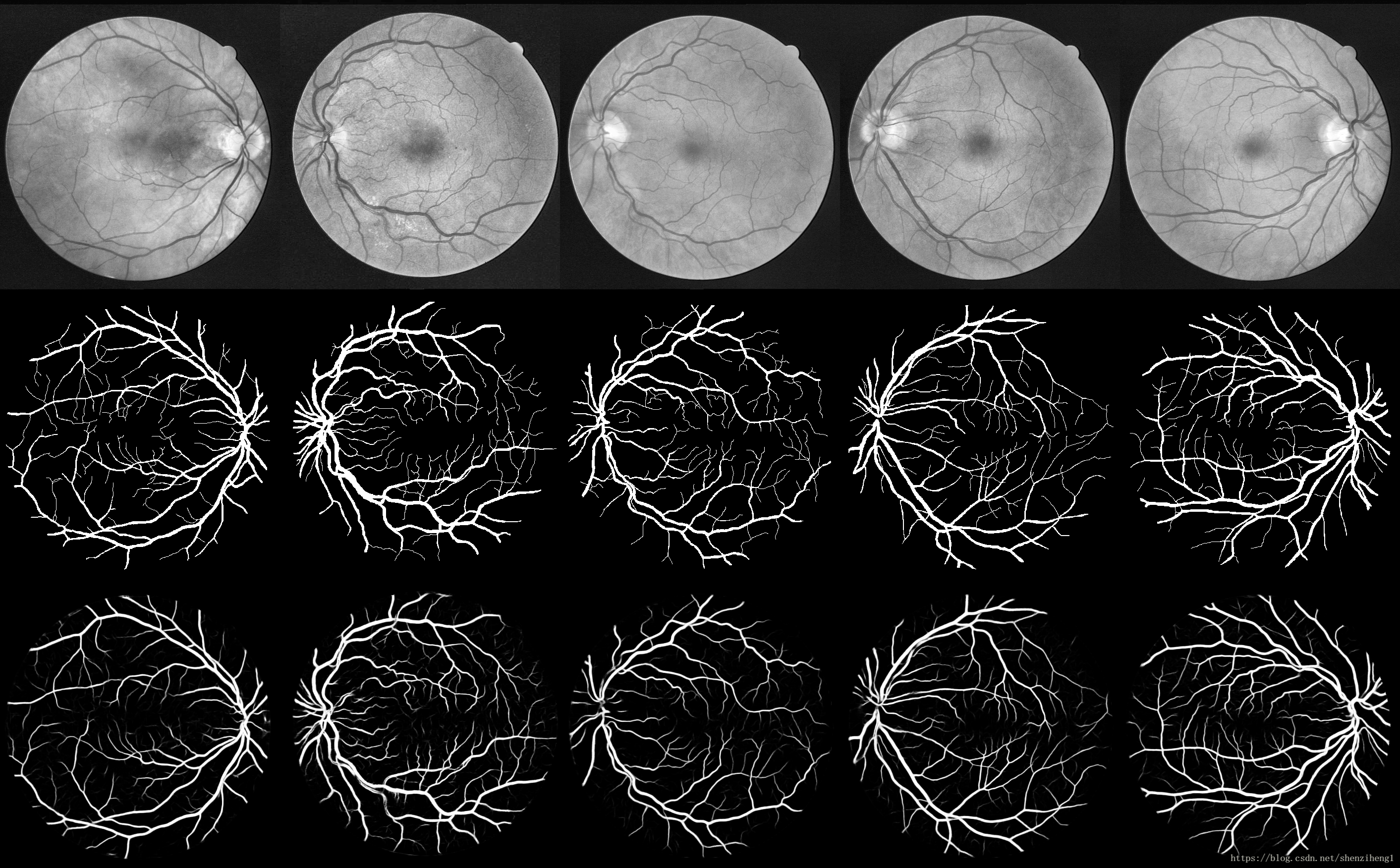
visualize(group_images(test_imgs_orig[0:20,:,:,:],5),'original').show() #显示所有的测试图像
visualize(group_images(test_border_masks[0:20,:,:,:],5),'borders').show()#显示所有的掩膜图像
visualize(group_images(img_truth[0:20,:,:,:],5),'gtruth').show() #显示所有的金标准图像

3. 图像分块、预测

patches_imgs_test = None
masks_test  = None
patches_masks_test = None
new_height = None
new_width = None
if average_mode == True:
    patches_imgs_test, new_height, new_width, masks_test = get_data_testing_overlap(
        DRIVE_test_imgs_original = DRIVE_test_imgs_original,  #original
        DRIVE_test_groudTruth = path_data + config.get('data paths', 'test_groundTruth'),  #masks
        Imgs_to_test = int(config.get('testing settings', 'full_images_to_test')),
        patch_height = patch_height,
        patch_width = patch_width,
        stride_height = stride_height,
        stride_width = stride_width
    )
else:
    patches_imgs_test, patches_masks_test = get_data_testing(
        DRIVE_test_imgs_original = DRIVE_test_imgs_original,  #original
        DRIVE_test_groudTruth = path_data + config.get('data paths', 'test_groundTruth'),  #masks
        Imgs_to_test = int(config.get('testing settings', 'full_images_to_test')),
        patch_height = patch_height,
        patch_width = patch_width,
    )

前者是采用覆盖式的图像块获取方法，后者就是简单的拼凑式。

#================ Run the prediction of the patches ==================================
best_last = config.get('testing settings', 'best_last')
#加载已经训练好的模型 和 相关的权重
model = model_from_json(open(path_experiment+name_experiment +'_architecture.json').read())
model.load_weights(path_experiment+name_experiment + '_'+best_last+'_weights.h5')
#进行模型预测
predictions = model.predict(patches_imgs_test, batch_size=32, verbose=1) # verbose = 1 采用进度条形式进行显示 
print ("predicted images size :")
print (predictions.shape)

#===== Convert the prediction arrays in corresponding images
pred_patches = pred_to_imgs(predictions, patch_height, patch_width, "original")

这里有一个非常重要的函数，就是pred_to_imgs, 后面我会专门写一遍博客仔细研究一下分块方法、整合方法、预测结果还原成图像以及可视化。

# 对于预测的数据将掩膜外的数据清零
kill_border(pred_imgs, test_border_masks)
## back to original dimensions
orig_imgs = orig_imgs[:,:,0:full_img_height,0:full_img_width]
pred_imgs = pred_imgs[:,:,0:full_img_height,0:full_img_width]
gtruth_masks = gtruth_masks[:,:,0:full_img_height,0:full_img_width]
print ("Orig imgs shape: " +str(orig_imgs.shape))
print ("pred imgs shape: " +str(pred_imgs.shape))
print ("Gtruth imgs shape: " +str(gtruth_masks.shape))

#可视化结果 对比预测 与 金标准
assert (orig_imgs.shape[0]==pred_imgs.shape[0] and orig_imgs.shape[0]==gtruth_masks.shape[0])
N_predicted = orig_imgs.shape[0]
group = N_visual
assert (N_predicted%group==0)
for i in range(int(N_predicted/group)):
    orig_stripe = group_images(orig_imgs[i*group:(i*group)+group,:,:,:],group)
    masks_stripe = group_images(gtruth_masks[i*group:(i*group)+group,:,:,:],group)
    pred_stripe = group_images(pred_imgs[i*group:(i*group)+group,:,:,:],group)
    total_img = np.concatenate((orig_stripe,masks_stripe,pred_stripe),axis=0)
    visualize(total_img,path_experiment+name_experiment +"_Original_GroundTruth_Prediction"+str(i)).show()

4. 对深度模型进行评价

作者主要用了sklearn模块的中模型评价函数， sklearn.metrics。

 

• sklearn.metrics.roc_curve ： 受试者工作曲线/准确性评价

sklearn.metrics.roc_curve(y_true, y_score, pos_label=None, sample_weight=None, drop_intermediate=True)

计算受试者工作特性曲线Receiver Operating Characteristic， ROC。只能应用于二分类问题。

ROC曲线指受试者工作特征曲线/接收器操作特性(receiver operating characteristic，ROC)曲线,是反映灵敏性和特效性连续变量的综合指标,是用构图法揭示敏感性和特异性的相互关系，它通过将连续变量设定出多个不同的临界值，从而计算出一系列敏感性和特异性。ROC曲线是根据一系列不同的二分类方式（分界值或决定阈），以真正例率（也就是灵敏度）（True Positive Rate,TPR）为纵坐标，假正例率（1-特效性）（False Positive Rate,FPR）为横坐标绘制的曲线。

ROC观察模型正确地识别正例的比例与模型错误地把负例数据识别成正例的比例之间的权衡。TPR的增加以FPR的增加为代价。ROC曲线下的面积是模型准确率的度量，AUC（Area under roccurve）。

纵坐标：真正率（True Positive Rate , TPR）或灵敏度（sensitivity）：TPR = TP /（TP + FN）  （正样本预测结果数 / 正样本实际数）

横坐标：假正率（False Positive Rate , FPR）：FPR = FP /（FP + TN） （被预测为正的负样本结果数 /负样本实际数）

该函数返回这三个变量：fpr,tpr,和阈值thresholds; 这里理解thresholds: 分类器的一个重要功能“概率输出”，即表示分类器认为某个样本具有多大的概率属于正样本（或负样本）。

Score表示每个测试样本属于正样本的概率。接下来，从高到低，依次将Score值作为阈值threshold，当测试样本属于正样本的概率大于或等于这个threshold时，我们认为它为正样本，否则为负样本。每次选取一个不同的threshold，我们就可以得到一组FPR和TPR，即ROC曲线上的一点。当我们将threshold设置为1和0时，分别可以得到ROC曲线上的(0,0)和(1,1)两个点。将这些(FPR,TPR)对连接起来，就得到了ROC曲线。当threshold取值越多，ROC曲线越平滑。其实，我们并不一定要得到每个测试样本是正样本的概率值，只要得到这个分类器对该测试样本的“评分值”即可（评分值并不一定在(0,1)区间）。评分越高，表示分类器越肯定地认为这个测试样本是正样本，而且同时使用各个评分值作为threshold。

#====== Evaluate the results
print ("\n\n========  Evaluate the results =======================")
# 只预测FOV内部的图像
y_scores, y_true = 
	pred_only_FOV(pred_imgs,gtruth_masks, test_border_masks)
print ("Calculating results only inside the FOV:")
print ("y scores pixels: " +str(y_scores.shape[0]) +
        " (radius 270: 270*270*3.14==228906), including background around retina: " +
		str(pred_imgs.shape[0]*pred_imgs.shape[2]*pred_imgs.shape[3]) +" (584*565==329960)"
print ("y true pixels: " +str(y_true.shape[0]) +
		" (radius 270: 270*270*3.14==228906), including background around retina: " +
		str(gtruth_masks.shape[2]*gtruth_masks.shape[3]*gtruth_masks.shape[0])+" (584*565==329960)"

# ROC曲线下的面积
fpr, tpr, thresholds = roc_curve((y_true), y_scores)
AUC_ROC = roc_auc_score(y_true, y_scores)
# test_integral = np.trapz(tpr,fpr) #trapz is numpy integration
print ("\n Area under the ROC curve: " +str(AUC_ROC))
roc_curve =plt.figure()
plt.plot(fpr,tpr,'-',label='Area Under the Curve (AUC = %0.4f)' % AUC_ROC)
plt.title('ROC curve')
plt.xlabel("FPR (False Positive Rate)")
plt.ylabel("TPR (True Positive Rate)")
plt.legend(loc="lower right")
plt.savefig(path_experiment+"ROC.png")

 

• sklearn.metrics.precision_recall_curve：精确度-召回率曲线

以推荐算法为例：

A：检索到的，相关的                    （搜到的也想要的）
B：检索到的，但是不相关的           （搜到的但没用的）
C：未检索到的，但却是相关的        （没搜到，然而实际上想要的）
D：未检索到的，也不相关的           （没搜到也没用的）
如果我们希望：被检索到的内容越多越好，是追求“查全率”，即A/(A+C)，越大越好。

如果我们希望：检索到的文档中，真正想要的、也就是相关的越多越好，不相关的越少越好，是追求“准确率”，即A/(A+B)，越大越好。

#Precision-recall curve
precision, recall, thresholds = precision_recall_curve(y_true, y_scores)
precision = np.fliplr([precision])[0]  #so the array is increasing (you won't get negative AUC)
recall = np.fliplr([recall])[0]  #so the array is increasing (you won't get negative AUC)
AUC_prec_rec = np.trapz(precision,recall)
print "\nArea under Precision-Recall curve: " +str(AUC_prec_rec)
prec_rec_curve = plt.figure()
plt.plot(recall,precision,'-',label='Area Under the Curve (AUC = %0.4f)' % AUC_prec_rec)
plt.title('Precision - Recall curve')
plt.xlabel("Recall")
plt.ylabel("Precision")
plt.legend(loc="lower right")
plt.savefig(path_experiment+"Precision_recall.png")

• sklearn.metrics.confusion_matrix ： 混淆矩阵

混淆矩阵是对有监督学习分类算法准确率进行评估的工具。通过将模型预测的数据与测试数据进行对比，使用各种指标对模型的分类效果进行度量。

#Confusion matrix
threshold_confusion = 0.5
print ("\nConfusion matrix:  Costum threshold (for positive) of " +str(threshold_confusion))
y_pred = np.empty((y_scores.shape[0]))
for i in range(y_scores.shape[0]):
    if y_scores[i]>=threshold_confusion:
        y_pred[i]=1
    else:
        y_pred[i]=0
confusion = confusion_matrix(y_true, y_pred)
print (confusion)
accuracy = 0
if float(np.sum(confusion))!=0:
    accuracy = float(confusion[0,0]+confusion[1,1])/float(np.sum(confusion))
print ("Global Accuracy: " +str(accuracy))
specificity = 0
if float(confusion[0,0]+confusion[0,1])!=0:
    specificity = float(confusion[0,0])/float(confusion[0,0]+confusion[0,1])
print ("Specificity: " +str(specificity))
sensitivity = 0
if float(confusion[1,1]+confusion[1,0])!=0:
    sensitivity = float(confusion[1,1])/float(confusion[1,1]+confusion[1,0])
print ("Sensitivity: " +str(sensitivity))
precision = 0
if float(confusion[1,1]+confusion[0,1])!=0:
    precision = float(confusion[1,1])/float(confusion[1,1]+confusion[0,1])
print ("Precision: " +str(precision))

• sklearn.metrics. jaccard_similarity_score : jacaard相似度

jaccard index又称为jaccard similarity coefficient用于比较有限样本集之间的相似性和差异性。定义：

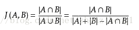
给定两个集合A,B jaccard 系数定义为A与B交集的大小与并集大小的比值。jaccard值越大说明相似度越高。

#Jaccard similarity index
jaccard_index = jaccard_similarity_score(y_true, y_pred, normalize=True)
print ("\nJaccard similarity score: " +str(jaccard_index))

• sklearn.metrics.f1_score

F1-score:  是准确率与召回率的综合。 可以认为是平均效果

#F1 score
F1_score = f1_score(y_true, y_pred, labels=None, average='binary', sample_weight=None)
print ("\nF1 score (F-measure): " +str(F1_score))

 

最后保存数据结果。

#Save the results
file_perf = open(path_experiment+'performances.txt', 'w')
file_perf.write("Area under the ROC curve: "+str(AUC_ROC)
                + "\nArea under Precision-Recall curve: " +str(AUC_prec_rec)
                + "\nJaccard similarity score: " +str(jaccard_index)
                + "\nF1 score (F-measure): " +str(F1_score)
                +"\n\nConfusion matrix:"
                +str(confusion)
                +"\nACCURACY: " +str(accuracy)
                +"\nSENSITIVITY: " +str(sensitivity)
                +"\nSPECIFICITY: " +str(specificity)
                +"\nPRECISION: " +str(precision)
                )
file_perf.close()