


极端梯队提升 Extreme Gradient Boosting
贪婪函数逼近 Greedy Function Approximation
梯队提升树 gradient boosted trees
监督学习 Supervised Learning
模型和参数 Model and Parameters
线性回归预测为例 linear model prediction :
y ^ i = ∑ j θ j x i j \hat{y}_i = \sum_j \theta_j x_{ij} y^i=∑jθjxij
模型解读: a linear combination of weighted input features 加权输入特征的线性组合
预测值含义: depending on the task, i.e., regression or classification
参数: are the undetermined part that we need to learn from data
目标函数 objective function :
训练的目的: The task of training the model amounts to finding the best parameters θ that best fit the training data xi and labels yi
目标函数的用途: define the objective function to measure how well the model fit the training data.
目标函数的定义objective function
training loss and regularization term:
obj ( θ ) = L ( θ ) + Ω ( θ ) \text{obj}(\theta) = L(\theta) + \Omega(\theta) obj(θ)=L(θ)+Ω(θ)
包含两部分:training loss and regularization term
训练损失函数training loss function
训练损失函数的用途:
我们的模型对训练数据的预测性
measures how predictive our model is with respect to the training data
均方误差mean squared error
公式定义:
L ( θ ) = ∑ i ( y i − y ^ i ) 2 L(\theta) = \sum_i (y_i-\hat{y}_i)^2 L(θ)=∑i(yi−y^i)2
逻辑损失函数 ogistic loss function
L ( θ ) = ∑ i [ y i ln ( 1 + e − y ^ i ) + ( 1 − y i ) ln ( 1 + e y ^ i ) ] L(\theta) = \sum_i[ y_i\ln (1+e^{-\hat{y}_i}) + (1-y_i)\ln (1+e^{\hat{y}_i})] L(θ)=∑i[yiln(1+e−y^i)+(1−yi)ln(1+ey^i)]
正则化项 regularization term
意义: 控制模型的复杂性,这有助于我们避免过度拟合
controls the complexity of the model, to avoid overfitting
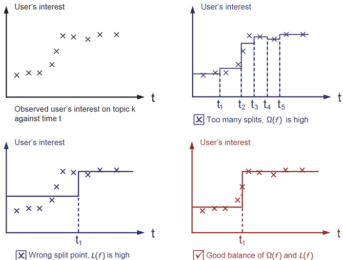
平衡损失函数和正则化项 bias-variance tradeoff
too many spits, 正则化项函数值高.
wrong split point, 损失函数数值高.
两者之间的权衡也称为机器学习中的bias-variance tradeoff 偏差-方差权衡。
决策树集合 Decision Tree Ensembles
分类树,回归树的集合 classification trees, regression trees
CART案例
输入: age,gender,occupation 年龄,性别,职业
输出: prediction score in each leaf
使用集合模型的原因:
- a single tree is not strong enough to be used in practice. What is actually used is the ensemble model, which sums the prediction of multiple trees together.
- 单棵树的强度不足以在实践中使用。实际使用的是集合模型,它将多个树的预测相加在一起。
另一个好处:
- two trees try to complement each other
- 一个重要的事实是这两棵树试图相互补充
数学公式
预测模型:
y ^ i = ∑ k = 1 K f k ( x i ) , f k ∈ F \hat{y}_i = \sum_{k=1}^K f_k(x_i), f_k \in \mathcal{F} y^i=∑k=1Kfk(xi),fk∈F
- K is the number of trees
- f is a function in the functional space \mathcal{F},
and F \mathcal{F} F is the set of all possible CARTs
所有可能的CART的集合
目标函数:
obj ( θ ) = ∑ i n l ( y i , y ^ i ) + ∑ k = 1 K Ω ( f k ) \text{obj}(\theta) = \sum_i^n l(y_i, \hat{y}_i) + \sum_{k=1}^K \Omega(f_k) obj(θ)=∑inl(yi,y^i)+∑k=1KΩ(fk)
提升树 Tree Boosting
所有监督学习模型训练都是如此:定义目标函数并对其进行优化!
for all supervised learning models: define an objective function and optimize it!
obj = ∑ i = 1 n l ( y i , y ^ i ( t ) ) + ∑ i = 1 t Ω ( f i ) \text{obj} = \sum_{i=1}^n l(y_i, \hat{y}_i^{(t)}) + \sum_{i=1}^t\Omega(f_i) obj=∑i=1nl(yi,y^i(t))+∑i=1tΩ(fi)
加法训练 Additive Training
关于 f i f_i fi
y ^ i = ∑ k = 1 K f k ( x i ) , f k ∈ F \hat{y}_i = \sum_{k=1}^K f_k(x_i), f_k \in \mathcal{F} y^i=∑k=1Kfk(xi),fk∈F
- f is a function in the functional space
F
\mathcal{F}
F,
and \mathcal{F} is the set of all possible CARTs
f
i
f_i
fi 每个都包含树的结构和叶子的分数
一次学习所有树是难以处理的
我们使用一个加法策略:修复我们学到的东西,并一次添加一个新树
预测值为
y
^
i
(
t
)
\hat{y}_i^{(t)}
y^i(t)
KaTeX parse error: Expected 'EOF', got '&' at position 16: hat{y}_i^{(0)} &̲= 0\\ \hat{y}_i…
目标函数:
$\text{obj}^{(t)} & = \sum_{i=1}^n l(y_i, \hat{y}i^{(t)}) + \sum{i=1}^t\Omega(f_i) \$
KaTeX parse error: Expected 'EOF', got '&' at position 1: &̲ = \sum_{i=1}^n…
如果我们考虑使用均方误差mean squared error(MSE)作为我们的损失函数,那么目标就变成了
目标函数为
$\text{obj}^{(t)} & = \sum_{i=1}^n (y_i - (\hat{y}i^{(t-1)} + f_t(x_i)))^2 + \sum{i=1}^t\Omega(f_i) \$
KaTeX parse error: Expected 'EOF', got '&' at position 1: &̲ = \sum_{i=1}^n…
MSE的形式是友好的,具有一阶项(通常称为残差)和二次项
a first order term (usually called the residual) and a quadratic term
我们将损失函数的泰勒展开式提升到二阶:
we take the Taylor expansion of the loss function up to the second order:
obj
(
t
)
=
∑
i
=
1
n
[
l
(
y
i
,
y
^
i
(
t
−
1
)
)
+
g
i
f
t
(
x
i
)
+
1
2
h
i
f
t
2
(
x
i
)
]
+
Ω
(
f
t
)
+
c
o
n
s
t
a
n
t
\text{obj}^{(t)} = \sum_{i=1}^n [l(y_i, \hat{y}_i^{(t-1)}) + g_i f_t(x_i) + \frac{1}{2} h_i f_t^2(x_i)] + \Omega(f_t) + \mathrm{constant}
obj(t)=∑i=1n[l(yi,y^i(t−1))+gift(xi)+21hift2(xi)]+Ω(ft)+constant
其中 gi 和 hi 被定义为
$g_i &= \partial_{\hat{y}_i^{(t-1)}} l(y_i, \hat{y}_i^{(t-1)})\$
KaTeX parse error: Expected 'EOF', got '&' at position 5: h_i &̲= \partial_{\ha…
在我们删除所有常量后,步骤中的具体目标 t 变
∑ i = 1 n [ g i f t ( x i ) + 1 2 h i f t 2 ( x i ) ] + Ω ( f t ) \sum_{i=1}^n [g_i f_t(x_i) + \frac{1}{2} h_i f_t^2(x_i)] + \Omega(f_t) ∑i=1n[gift(xi)+21hift2(xi)]+Ω(ft)
  这成为我们对新树的优化目标。该定义的一个重要优点是目标函数的值仅取决于gi 和 hi。
  这就是XGBoost如何支持自定义损失函数。
模型复杂度 Model Complexity 正则项
定义树的复杂性 \Omega(f)
完善树的定义f(x)
f
t
(
x
)
=
w
q
(
x
)
,
w
∈
R
T
,
q
:
R
d
→
{
1
,
2
,
⋯
,
T
}
f_t(x) = w_{q(x)}, w \in R^T, q:R^d\rightarrow \{1,2,\cdots,T\}
ft(x)=wq(x),w∈RT,q:Rd→{1,2,⋯,T}
- w 是叶子上的分数矢量, q 是一个将每个数据点分配给相应叶子的函数,和 T是叶子的数量
在XGBoost中,我们将复杂性定义为
Ω
(
f
)
=
γ
T
+
1
2
λ
∑
j
=
1
T
w
j
2
\Omega(f) = \gamma T + \frac{1}{2}\lambda \sum_{j=1}^T w_j^2
Ω(f)=γT+21λ∑j=1Twj2
The Structure Score
在重新制定树模型后,我们可以用它来写出目标值t树为
KaTeX parse error: Expected 'EOF', got '&' at position 17: …ext{obj}^{(t)} &̲\approx \sum_{i…
I j = { i ∣ q ( x i ) = j } I_j = \{i|q(x_i)=j\} Ij={i∣q(xi)=j} 是分配给的数据点的索引集 j - 叶子
因为同一叶子上的所有数据点都得到相同的分数
我们可以通过定义来进一步压缩表达式
G j = ∑ i ∈ I j g i H j = ∑ i ∈ I j h i G_j = \sum_{i\in I_j} g_i H_j = \sum_{i\in I_j} h_i Gj=∑i∈IjgiHj=∑i∈Ijhi
obj ( t ) = ∑ j = 1 T [ G j w j + 1 2 ( H j + λ ) w j 2 ] + γ T \text{obj}^{(t)} = \sum^T_{j=1} [G_jw_j + \frac{1}{2} (H_j+\lambda) w_j^2] +\gamma T obj(t)=∑j=1T[Gjwj+21(Hj+λ)wj2]+γT
- wj 形式相互独立
G
j
w
j
+
1
2
(
H
j
+
λ
)
w
j
2
G_jw_j+\frac{1}{2}(H_j+\lambda)w_j^2
Gjwj+21(Hj+λ)wj2 是二次的
也是最好的 wj 对于给定的结构 q(x) 我们可以得到的最好的客观减少是
KaTeX parse error: Expected 'EOF', got '&' at position 10: w_j^\ast &̲= -\frac{G_j}{H…
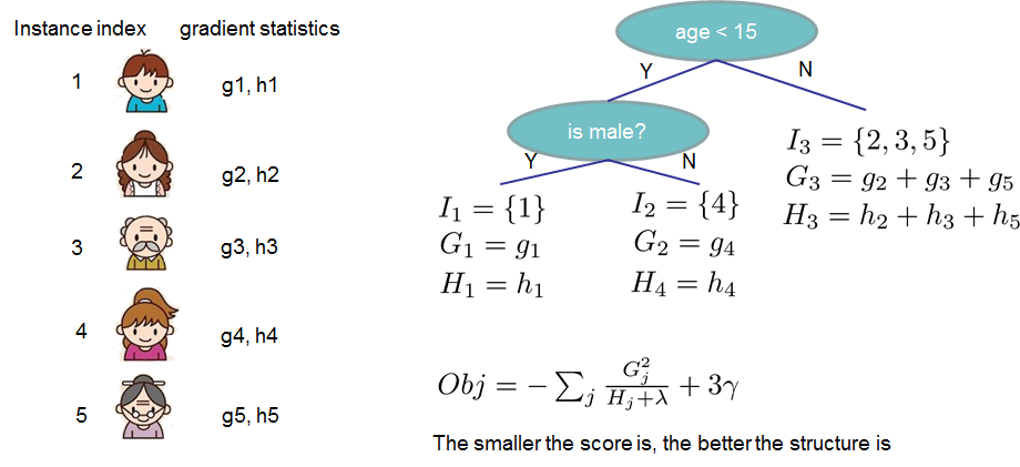
the smaller the sore is ,the better the structure is
Learn the tree structure
理想情况下我们会列举所有可能的树并选择最好的树。在实践中,这是难以处理的,因此我们将尝试一次优化树的一个级别。具体来说,我们尝试将一片叶子分成两片叶子,它获得的分数是
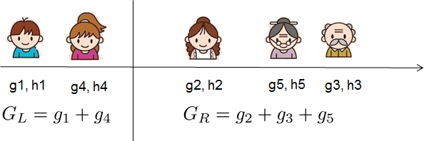
G a i n = 1 2 [ G L 2 H L + λ + G R 2 H R + λ − ( G L + G R ) 2 H L + H R + λ ] − γ Gain = \frac{1}{2} \left[\frac{G_L^2}{H_L+\lambda}+\frac{G_R^2}{H_R+\lambda}-\frac{(G_L+G_R)^2}{H_L+H_R+\lambda}\right] - \gamma Gain=21[HL+λGL2+HR+λGR2−HL+HR+λ(GL+GR)2]−γ
该公式可以分解为1)新左叶上的分数2)新右叶上的分数3)原叶上的分数4)附加叶上的正则化。
看到一个重要的事实:如果增益小于γ,我们最好不要添加该分支。这正是基于树的模型中的修剪技术!
对于实值数据,我们通常希望搜索最佳分割。为了有效地执行此操作,我们将所有实例按排序顺序放置,如下图所示。


 350
350

 被折叠的 条评论
为什么被折叠?
被折叠的 条评论
为什么被折叠?
 到【灌水乐园】发言


