Medians and Order Statistics - Introduction to Algorithm - Summary of Chapter 9

Introduction of Chapter

The ith order statistic of a set of n elements is the ith smallest element.

A median, informally, is the “halfway point” of the set.
If the number of set if even , the lower median is $\lfloor(n+1)/2\rfloor$ smallest element, and the upper median is $\lceil(n+1)/2\rceil$ smallest element.

---

Minimum and maximum

Minimum (A)
    min = A[1]
    for i=2 to A.length
        if min > A[i]
            min = A[i]
    return min

Simultaneous minimum and maximum
We compare pairs of elements from the input first with each other, and then we compare the smaller with the current minimum and the larger to the current maximum, at a cost of 3 comparisons for every 2 elements. Finding both the minimum and the maximum using at most $3\lfloor n/2\rfloor$ comparisons.

---

Selection in expected linear time

Randomized-Select(A, p, r, i)
    if p==r
        return A[p]
    q = Randomized-Partition (A, p, r)
    k = q-p+1
    if i==k
        return A[q]
    elseif i<k
        return Randomized-Select (A, p, q-1, i)
    else return Randomized-Select (A, q+1, r, i-k)

The expected running time for Randomized-Select is $\Theta(n)$

The worst-case running time for Randomized-Select is $\Theta(n^2)$ even to find the minimum, because we could be extremely unlucky and always partition around the largest remaining element, and partitioning takes $\Theta(n)$ time.

---

Selection in worst-case linear time

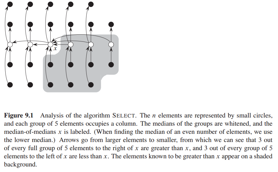
The SELECT algorithm determines the ith smallest of an input array of $n > 1$ distinct elements by executing the following steps. (If $n = 1$, then SELECT merely returns its only input value as the ith smallest.)

1. Divide the n elements of the input array into $\lfloor n/5\rfloor$ groups of 5 elements each and at most one group made up of the remaining $n \mod 5$ elements.
2. Find the median of each of the $\lceil n/5\rceil$ groups by first insertion-sorting the elements of each group (of which there are at most 5) and then picking the median from the sorted list of group elements.
3. Use SELECT recursively to find the median x of the $\lceil n/5\rceil$ medians found in step 2. (If there are an even number of medians, then by our convention, x is the lower median.)
4. Partition the input array around the median-of-medians x using the modified version of PARTITION. Let k be one more than the number of elements on the low side of the partition, so that x is the kth smallest element and there are n-k elements on the high side of the partition.
5. If i = k, then return x. Otherwise, use SELECT recursively to find the ith smallest element on the low side if i < k, or the .(i-k)th smallest element on the high side if i > k.

---

Exercises

9.1.1
$\star$ Show that the second smallest of n elements can be found with $n + \lceil \lg n\rceil - 2$ comparisons in the worst case. (Hint: Also find the smallest element.)

We can compare the elements in a tournament fashion - we split them into pairs, compare each pair and then proceed to compare the winners in the same fashion. We need to keep track of each “match” the potential winners have participated in.

We select a winner in n - 1 matches. At this point, we know that the second smallest element is one of the $\lg{n}$ elements that lost to the smallest ­ each of them is smaller than the ones it has been compared to,(These $\lg n -1$ elements is the one of which was compared with the smallest one and was bear) prior to losing. In another $\lceil \lg{n} \rceil - 1$ comparisons we can find the smallest element out of those. This is the answer we are looking for.

---

9.1.2
$\star$ Prove the lower bound of $\lceil3n/2\rceil - 2$ comparisons in the worst case to find both the maximum and minimum of n numbers. (Hint: Consider how many numbers are potentially either the maximum or minimum, and investigate how a comparison affects these counts.)

We can optimize by splitting the input in pairs and comparing each pair. After $n/2$ comparisons, we have reduced the potential minimums and potential maximums to $n/2$ each. In that moment , which bigger ,which smaller is coming . Furthermore, the bigger one and the smaller one of first pair is viewed the maximum and the minimum in the algorithm beginning. There are two comparisions each of the $(n-1)$ remainder pair, the bigger one is compared with maximum and the smaller is compared with minimum.
The total number of comparisons is:
$n/2 + 2(n/2 - 1) = n/2 + n - 2 = 3n/2 - 2$
This assumes that n is even. If n is odd we need one additional comparison in order to determine whether the last element is a potential minimum or maximum. Hence the ceiling.

9.2.1
$\star$ Show that RANDOMIZED-SELECT never makes a recursive call to a 0-length array.

The are two cases where it appears that RANDOMIZED-SELECT can make a call to a 0-length array:

1. Line 8 with $k = 1$. But for this to happen, $i$ needs to be 0. And that cannot happen since the initial call is supposed to pass a nonzero $i$ and the recursive calls either pass $i$ unmodified or pass $i - k$ where $i > k$.
2. Line 9 with $q = r$. But for this to happen, $i$ must be greater than $k$, that is $i > q - p + 1 = r - p + 1$, that is, $i$ needs to be greater than the number of elements in the array. Initially that is not true and both recursive calls maintain an invariant that $i$ is less or equal to the number of elements in $A[p..q]$.

9.2.2
$\star$ Argue that the indicator random variable $X_k$ and the value
$T(\max(k-1,n-k))$ are independent

Picking the pivot in one partitioning does not affect the probabilities of the subproblem. That is, the call to RANDOM in RANDOMIZED-PARTITION produces a result, independent from the call in the next iteration.

9.2.3
$\star$ Write an iterative version of RANDOMIZED-SELECT.

#include <stdlib.h>

static int tmp;
#define EXCHANGE(a, b) { tmp = a; a = b; b = tmp; }

int randomized_partition(int *A, int p, int r);

int randomized_select(int *A, int p, int r, int i) {
    while (p < r - 1) {
        int q = randomized_partition(A, p, r);
        int k = q - p;

        if (i == k) {
            return A[q];
        } else if (i < k) {
            r = q;
        } else {
            p = q + 1;
            i = i - k - 1;
        }
    }

    return A[p];
}

int partition(int *A, int p, int r) {
    int x, i, j;

    x = A[r - 1];
    i = p;

    for (j = p; j < r - 1; j++) {
        if (A[j] < x) {
            EXCHANGE(A[i], A[j]);
            i++;
        }
    }

    EXCHANGE(A[i], A[r - 1]);

    return i;
}

int randomized_partition(int *A, int p, int r) {
    int pivot = rand() % (r - p) + p;
    EXCHANGE(A[pivot], A[r - 1]);
    return partition(A, p, r);
}

9.2.4
$\star$ Suppose we use RANDOMIZED-SELECT to select the minimum element of the array $A = \langle 3, 2, 9, 0, 7, 5, 4, 8, 6, 1 \rangle$. Describe a sequence of partitions that results in a worst-case performance of RANDOMIZED-SELECT.

This happens if all the elements get picked up in reverse order ­ that is, the first pivot chosen is 9, the second is 8, the third is 7 and so on.

---

9.3.1
$\star$ In the algorithm SELECT, the input elements are divided into groups of 5. Will the algorithm work in linear time if they are divided into groups of 7? Argue that SELECT does not run in linear time if groups of 3 are used.

Groups of 7
The algorithm will work if the elements are divided in groups of 7. On each partitioning, the minimum number of elements that are less than (or greater than) x will be:

$$4 \bigg(\bigg\lceil \frac{1}{2} \Big\lceil \frac{n}{7} \Big\rceil \bigg\rceil - 2 \bigg) \ge \frac{2n}{7} - 8$$
The partitioning will reduce the subproblem to size at most 5n/7 + 8. This yields the following recurrence:

$$T(n) = \begin{cases} O(1) & \text{ if } n < n_0 \\ T(\lceil n/7 \rceil) + T(5n/7 + 8) + O(n) & \text{ if } n \ge n_0 \end{cases}$$
We guess T(n) \le cn and bound the non-recursive term with an:

$$\begin{align} T(n) & \le c\lceil n/7 \rceil + c(5n/7 + 8) + an \\ & \le cn/7 + c + 5cn/7 + 8c + an \\ & = 6cn/7 + 9c + an \\ & = cn + (-cn/7 + 9c + an) \\ & \le cn \\ & = O(n) \end{align}$$
The last step holds when $(-cn/7 + 9c + an) \le 0$. That is:

$$-cn/7 + 9c + an \le 0 \\ \Downarrow \\ c(n/7 - 9) \ge an \\ \Downarrow \\ \frac{c(n - 63)}{7} \ge an \\ \Downarrow \\ c \ge \frac{7an}{n - 63}$$
By picking $n_0 = 126$ and $n \le n_0$, we get that $n/(n - 63) \le 2$. Then we just need $c \ge 14a$.

Groups of 3
The algorithm will not work for groups of three. The number of elements that are less than (or greater than) the median-of-medians is:

$$2 \bigg(\bigg\lceil \frac{1}{2} \Big\lceil \frac{n}{3} \Big\rceil \bigg\rceil - 2 \bigg) \ge \frac{n}{3} - 4$$
The recurrence is thus:

$$T(n) = T(\lceil n/3 \rceil) + T(2n/3 + 4) + O(n)$$
We’re going to prove that T(n) = \omega(n) using the substitution method. We guess that T(n) > cn and bound the non-recursive term with an.

$$\begin{align} T(n) & > c\lceil n/3 \rceil + c(2n/3 + 2) + an \\ & > cn/3 + c + 2cn/3 + 2c + an \\ & = cn + 3c + an & (c > 0, a > 0, n > 0)\\ & > cn \\ & = \omega(n) \end{align}$$
The calculation above holds for any $c > 0$.

9.3.2
Analyze SELECT to show that if $n\ge140$, then at least $\lceil n/4 \rceil$elements are greater than the median-of-medians x and at least dn=4e elements are less than x.

$$\frac{3n}{10} - 6 \ge \bigg\lceil \frac{n}{4} \bigg\rceil \\ \Downarrow \\ \frac{3n}{10} - 6 \ge \frac{n}{4} + 1 \\ \Downarrow \\ \frac{3n}{10} - 7 \ge \frac{n}{4} \\ \Downarrow \\ 12n - 280 \ge 10n \\ \Downarrow \\ 2n \ge 280 \\ \Downarrow \\ n \ge 140$$

9.3.3
$\star$ Show how quicksort can be made to run in O(nlgn) time in the worst case, assuming that all elements are distinct.

If we rewrite PARTITION to use the same approach as SELECT, it will perform in $O(n)$ time, but the smallest partition will be at least one-fourth of the input (for large enough $n$, as illustrated in exercise 9.3.2). This will yield a worst-case recurrence of:

$$T(n)=T(n/4)+T(3n/4)+O(n)$$
As of exercise 4.4.9, we know that this is $Θ(nlgn)$.

And that’s how we can prevent quicksort from getting quadratic in the worst case, although this approach probably has a constant that is too large for practical purposes.

Another approach would be to find the median in linear time (with SELECT) and partition around it. That will always give an even split.

9.3.4
$\star$ Suppose that an algorithm uses only comparisons to find the ith smallest element in a set of n elements. Show that it can also find the i−1 smaller elements and the n−i larger elements without performing any additional comparisons.

A strict proof might require a more advanced proof apparatus than I command (like graphs and adversary algorithms, for example?), so I will just sketch it briefly.

In order to determine the ith order statistic, any algorithm needs to establish in some way that there are i−1 elements smaller than the result and n−i elements larger than the result. We can visualize the algorithm as a directed graph, where all the elements are edges. Each comparison introduces a node from the smaller to the larger element. To produce a result, there must be i−1 elements that (transitively) point to the ith order statistic and n−i elements that the ith order statistic (transitively) points to. There cannot be more (property of the order statistics) and if there are less, then there are elements whose position in regard to the ith order statistic is undetermined.

In order to find the result, the algorithm needs to build the knowledge presented in such a graph and it can use it to return the sets of smaller and larger elements.

As an example, both algorithms presented in the chapter leave the array partitioned around the ith order statistic.

9.3.5
$\star$ Suppose that you have a “black-box” worst-case linear time median subroutine. Give a simple, linear-time algorithm that solves the selection problem for an arbitrary order statistic.

We find the median in linear time partition the array around it (again, in linear time). If the median index (always $⌈n/2⌉$) equals n we return the median. Otherwise, we recurse either in the lower or upper part of the array, adjusting n accordingly.

This yields the following recurrence:

$$T(n)=T(n/2)+O(n)$$
Applying the master method, we get an upper bound of $O(n)$.

int select (A, p, r, i)//return the ith smallest element in array A[p..r]
{
    if (r<=p)
        return A[p];
    int k, q;
    k = median (A, p, r);//k is the position of the A[(r-p+1)/2+p],median A[k]
    if (i==k)
        return A[i];
    else if (i<k)
        select (A, p, k-1, i);
    else select (A, k+1, r, i-k);
}

9.3.6
$\star$ The $k$th quantiles of an $n$-element set are $k - 1$ order statistics that divide the sorted set into $k$ equal-sized sets (to within 1). Give an $O(n\lg{k})$-time algorithm to list the $k$th quantiles of a set.

If $k = 1$ we return an empty list.
If $k$ is even, we find the median, partition around it, solve two similar subproblems of size $\lfloor n / 2 \rfloor$ and return their solutions plus the median.
If $k$ is odd, we find the $\lfloor k/2 \rfloor$ and $\lceil k/2 \rceil$ boundaries and the we reduce to two subproblems, each with size less than $n/2$. The worst case recurrence is:

$$T(n, k) = 2T(\lfloor k/2 \rfloor) + O(n)$$

Which is the desired bound ­ $O(n\lg{k})$.

This works easily when the number of elements is $ak + k - 1$ for a positive integer $a$. When they are a different number, some care with rounding needs to be taken in order to avoid creating two segments that differ by more than 1.

9.3.7
$\star$ Describe an $O(n)$-time algorithm that, given a set S of n distinct numbers and a positive integer k n, determines the k numbers in S that are closest to the median of S.

1. We find the median of the array in linear time
2. We find the distance of each other element to the median in linear time
3. We find the k-th order statistic of the distance, again, in linear time
4. We select only the elements that have distance lower than or equal to the k-th order statistic

9.3.8
$\star$ Let $X[1..n]$ and $Y [1..n]$ be two arrays, each containing n numbers already in sorted order. Give an $O(lg n)$time algorithm to find the median of all 2n elements in arrays X and Y .

1. If the two arrays are of length 1, we pick the lower of the two elements
2. We compares the two medians of the array
3. We take the lower part of the array with the greater median and the upper part of the array with the lesser median to a new smaller array with size of half. If each array has n elements, we take the first/last $\lfloor n/2 \rfloor$ elements
4. We solve the problem for the new arrays recursively

Let’s reason about why this works. Since we have $2n$ elements, we know that the length is an even number and we’re looking for a lower median. We need to observe that the median we’re looking for is between the medians of the two arrays. Let’s elaborate on that.

Assume that the median is at position k in array A. This means that there are k−1 elements less than the median in A and k−1 elements greater than the median in B. If $k<n/2$ then the median of A will be greater than the final median, but the median of B will be lesser than it. It’s the other way around for k≥n/2. Thus the median of the two arrays is always between the medians of each.

Step 3 removes the same number of elements from each array, half of which are greater than the median and half of which are less than it. This reduces the subproblem to two smaller arrays that are sorted and their elements have the same median.

9.3.9
$\star$ Professor Olay is consulting for an oil company, which is planning a large pipeline running east to west through an oil fields of n wells. The company wants to connect a spur pipeline from each well directly to the main pipeline along a shortest route (either north or south), as shown on Figure 9.2. Given the x- and y- coordinates of the wells, how should the professor pick the optimal location of the main pipeline, which would be the one that minimizes the total length of the spurs? Show how to determine the optimal location in linear time.

We just find the median of the y coordinates. The x coordinates are irrelevant. The pipeline between any two wellspring can not decide the length . because it is decided only by the positions of two well. The important thing is to make sure the number of well beside pipeline is equal.

Let’s assume that n is odd. There are ⌊n/2⌋ south of the median and the same amount of wells north of the median. Let the pipeline pass through the median. We shall reason about why this location is optimal.

Suppose we move the pipeline one meter north. This reduces the total pipe length with ⌊n/2⌋ meters for the pipes north of the median, but adds another ⌈n/2⌉ for the pipes south of median, including the median itself. The more we move north, the more the total pipe length will increase. The same reasoning holds if we move the main pipeline south.

If n is even, then any location between the lower and upper median is optimal.

---

Problems

9.1 Largest i numbers in sorted order
Given a set of n numbers, we wish to find the i largest in sorted order using a comparison based algorithm. Find the algorithm that implements each of the following methods with the best asymptotic worst-case running time, and analyze the running time of the algorithms in terms of n and i.

$\star$a. Sort the numbers, and list the i largest

We can sort with any of the nlgn algorithms, that is, merge sort or heap sort and then just take the first i elements linearly.
This will take $n\lg n +i$ time.

$\star$b. Build a max-priority queue from the numbers, and call EXTRACT-MAX i times

We can build the heap linearly and then take each of the largest i elements in logarithmic time.
This takes $n+i\lg n$.

$\star$c. Use an order-statistic algorithm to find the ith largest number, partition around that number, and sort the i largest numbers.

Let’s assume we use the SELECT algorithm from the chapter. We can find the ith order statistic and partition around it in n time and then we need to do a sort in $i\lg i$.
This takes $n+i\lg i$

9.2 Weighted median
$\star$ For $n$ distinct elements $x_1, x_2, \ldots, x_n$ with positive weights $w_1, w_2, \ldots, w_n$ such that $\sum_{i=1}^n w_i = 1$, the weighted (lower) median is the element $x_k$ satisfying

$$\sum_{x_i < x_k} w_i <\frac{1}{2}$$
and
$$\sum_{x_i > x_k} w_i \le \frac{1}{2}$$
For example, if the elments are $0.1, 0.35, 0.05, 0.1, 0.15, 0.05, 0.2$ and
each element equals its weight (that is, $w_i = x_i$ for $i = 1, 2, \ldots, 7$, then the median is $0.1$, but the weighted median is $0.2$.

$\star$ a. Argue that the median of $x_1, x_2, \ldots, x_n$ is the weighted median of $x_i$ with weights $w_i = 1/n$ for $i = 1, 2, \ldots, n$.

If the weights all elements are $1/n$, then the sum of the weights of the elements, smaller than the median, is $\lfloor \frac{n - 1}{2} \rfloor \frac{1}{n}$ and the sum of the weights of the larger elements is $\lceil \frac{n - 1}{2} \rceil \frac{1}{n}$. This satisfies the condition for weighted median. Furthermore, choosing a smaller or greater value will not hold in the condition

$\star$ b. Show how to compute the weighted median of $n$ elements in $O(n\lg{n})$ worst-case time using sorting.

1. Sort the array
2. Start walking the array from left to right, accumulating the weights of the elements encountered
3. The first element with accumulated weight $w \ge 1/2$ is the weighted median

$\star$ c. Show how to compute the weighted median in $\Theta(n)$ worst-case time using a linear-time median algorithm such as SELECT from Section 9.3.

It’s a very similar to SELECT. In the step 4, we partition the whole array into two part by the median of median x. Then we sum the weights in the lower part of the array and the weights in the upper part. If they fulfill the condition, we have our weighted median. Otherwise we find it recursively in one of two part .There is a place worthy to notice that the recursive range is [q..r], but we compute the part weight sum in [1..A.length] every time.

$\star$ d. Argue that the weighted median is a best solution for the 1-dimensional post-office location problem, in which points are simply real numbers and the distance between points a and b is $d(a,b)=|a−b|$.

I’ll present an informal argument, since it is convincing enough. A more formal one can be found in the instructor’s manual.

The situation is similar to exercise 9.3.8. Let’s assume that we pick the weighted median as the solution and then start moving left or right. As we move away from the weighted median (in any direction), we’re moving towards elements with combined weight less than 1/2 and away from elements wight combined weight greater than 1/2. Every “step” we take, we’re increasing the total distance.

$\star$ e. Find the best solution for the 2-dimensional post-office location problem, in which the points are $(x,y)$ coordinate pairs and the distance between points $a = (x_1, y_1)$ and $b = (x_2, y_2)$ is the Manhattan distance given by $d(a, b) = |x_1 - x_2| + |y_1 - y_2|$.

The solution is finding $(x_m, y_m)$ where those are the weighted medians of
the $x$- and $y$- coordinates.

I’m not even going to start proving this formally, since it requires
mathematics above my current comfort level. Reasoning informally, by the definition of Manhattan distance, the $x$ coordinates and the $y$ coordinates are independent ­ we can rearrange the $x$ in any way we want, without affecting the $y$ coordinate of the solution and vice-versa.

9.3 Small order statistics
We showed that the worst-case number $T(n)$ of comparisons used by SELECT to select the ith order statistic from n numbers satisfies $T(n)=Θ(n)$, but the constant hidden by the $Θ$-notation is rather large. When $i$ is small relative to $n$, we can implement a different procedure that uses SELECT as a subroutine but makes fewer comparisons in the worst case.

$\star$ a. Describe an algorithm that uses $U_i(n)$ comparisons to find the ith smallest of n elements, where

$$U_i(n) = \begin{cases} T(n) & \text{if } i \ge n/2 \\ \lfloor n/2 \rfloor + U_i(\lceil n/2 \rceil) + T(2i) & \text{otherwise} \end{cases}$$
(Hint: Begin with $⌊n/2⌋$ disjoint pairwise comparisons, and recurse on the set containing the smaller element from each pair.)

This is a modified version of SELECT. Not only it finds the ith order statistic, but it also partitions the array, thus finding the i−1 smaller elements.

1. If $i≥n/2$, we just use SELECT
2. Otherwise, split the array in pairs and compare each pair.
3. We take the smaller elements of each pair, but keep track of the other one.
4. We recursively find the first i elements among the smaller elements
5. The ith order statistic is among the pairs containing the smaller elements we found in the previous step. We call SELECT on those 2i elements. That’s the final answer.

Just picking the smaller element of each pair is not enough. For example, if we’re looking for the 2nd order statistic and our pairs are 1, 2. 3, 4. 5, 6. 7, 8. 9, 10. the answer is in the larger part of the first pair. That’s why we need to keep track and later perform SELECT on 2i elements.

Steps 1-4 can be implemented in place by modifying the algorithm to put the larger elements of the pairs on the inactive side of the pivot and modifying PARTITION to swap the elements on the inactive side every time it swaps elements on the active side. More details can be found in the Instructor’s Manual.

$\star$ b. Show that, if $i < n/2$, then $U_i(n) = n + O(T(2i)\lg(n/i))$.

$$\begin{align} U_i(n) &= \lfloor n/2 \rfloor + U_i(\lceil n/2 \rceil) + T(2i) \\ &= \lfloor n/2 \rfloor + \lceil n/2 \rceil + O(T(2i)\lg(\lfloor n/2 \rfloor / i)) + T(2i) \\ &= n + O(T(2i)\lg(n/i)) + O(1) \\ &= n + O(T(2i)\lg(n/i)) \end{align}$$
This is a bit more sloppy that doing it with the substitution method, but that feels like grunt work to me at this point.

$\star$ d. Show that, if $i$ is a constant less than $n/2$, then $U_i(n) = n + O(\lg{n})$.

$$\begin{align} U_i(n) &= n + O(T(2i)\lg(n/i)) \\ &= n + O(O(1)\lg(n/i)) \\ &= n + O(\lg{n} - \lg{i}) \\ &= n + O(\lg{n} - O(1)) \\ &= n + O(\lg{n}) \end{align}$$

$\star$ e. Show that, if $i = n/k$ for $k \ge 2$, then $U_i(n) = n + O(T(2n/k)\lg{k})$.

$$\begin{align} U_i(n) &= n + O(T(2i)\lg(n/i)) \\ &= n + O(T(2n/k)\lg(n/(n/k))) \\ &= n + O(T(2n/k)\lg{k}) \\ \end{align}$$

9.4 Alternative analysis of randomized selection
$\star$ In this problem, we use indicator random variables to analyze the RANDOMIZED-SELECT procedure in a manner akin to our analysis of RANDOMIZED-QUICKSORT in section 7.4.2.

As in the quicksort analysis, we assume that all the elements are distinct, and we rename the elements of the input array A as z_1, z_2, \ldots, z_n, where z_i is the ith smallest element. Thus, the call RANDOMIZED-SELECT(A,1,n,k) returns z_k.

For $i \le i < j \le n$, let $X_{ijk} = I \{z_i \text{ is compared with } z_j \text{ sometime during the execution of the algorithm to find } z_k \}$

$\star$ a. Give an exact expression for $E[X_{ijk}]$. (Hint: Your expression may have different values, depending on the values of i, j, and k.)

The situation is very similar to the quicksort analysis, although k matters. $z_i$and $z_j$ will be compared if one of them is the first element to get picked as a pivot in the smallest interval containing i, j and k. The exact expression depends on the position of k in regards to the other two:

$$E[X_{ijk}] = \begin{cases} 1 / (k - i + 1)*2 & \text{if } i < j \le k \\ 1 / (j - i + 1)*2 & \text{if } i \le k \le j \\ 1 / (j - k + 1)*2 & \text{if } k \le i < j \end{cases}$$

$\star$ b. Let $X_k$ denote the total number of comparisons between elements of array A when finding $z_k$. Show that

$$E[X_k] \le 2 \bigg( \sum_{i=1}^k \sum_{j=k}^n \frac{1}{j - i + 1} + \sum_{j=k+1}^n \frac{j - k - 1}{j - k + 1} + \sum_{i=1}^{k-2} \frac{k - i - 1}{k - i + 1} \bigg)$$

It’s a long derivation:

$$\begin{align} E[X_k] &= \sum_{i=1}^{n-1} \sum_{j=i+1}^n E[X_{ijk}] \\ &= \sum_{i=1}^k \sum_{j=i+1}^n E[X_{ijk}] + \sum_{i=k+1}^{n-1} \sum_{j=i+1}^n E[X_{ijk}] \\ &= \sum_{i=1}^k \bigg(\sum_{j=i+1}^{k-1}E[X_{ijk}] + \sum_{j=k}^nE[X_{ijk}] \bigg) + \sum_{i=k+1}^{n-1}\sum_{j=i+1}^nE[X_{ijk}] \\ &= \sum_{i=1}^k \sum_{j=i+1}^{k-1} E[X_{ijk}] + \sum_{i=1}^k \sum_{j=k}^n E[X_{ijk}] + \sum_{i=k+1}^{n-1} \sum_{j=i+1}^n E[X_{ijk}] \\ &= \sum_{i=1}^{k-2} \sum_{j=i+1}^{k-1} E[X_{ijk}] + \sum_{i=1}^k \sum_{j=k}^n E[X_{ijk}] + \sum_{i=k+1}^{n-1} \sum_{j=i+1}^n E[X_{ijk}] \\ &= \sum_{i=1}^{k-2} \sum_{j=i+1}^{k-1} \frac{2}{k - i + 1} + \sum_{i=1}^k \sum_{j=k}^n \frac{2}{j - i + 1} + \sum_{i=k+1}^{n-1} \sum_{j=i+1}^n \frac{2}{j - k + 1} \\ &= 2\bigg( \sum_{i=1}^k \sum_{j=k}^n \frac{1}{j - i + 1} + \sum_{i=k+1}^{n-1} \sum_{j=i+1}^n \frac{1}{j - k + 1} + \sum_{i=1}^{k-2} \sum_{j=i+1}^{k-1} \frac{1}{k - i + 1} \bigg) \\ &= 2\bigg( \sum_{i=1}^k \sum_{j=k}^n \frac{1}{j - i + 1} + \sum_{i=k+1}^{n-1} \sum_{j=i+1}^n \frac{1}{j - k + 1} + \sum_{i=1}^{k-2} \frac{k - i - 1}{k - i + 1} \bigg) \\ &= 2\bigg( \sum_{i=1}^k \sum_{j=k}^n \frac{1}{j - i + 1} + \sum_{j=k+2}^n \sum_{i=k+1}^{j-1} \frac{1}{j - k + 1} + \sum_{i=1}^{k-2} \frac{k - i - 1}{k - i + 1} \bigg) & \text{(note below)} \\ &= 2\bigg( \sum_{i=1}^k \sum_{j=k}^n \frac{1}{j - i + 1} + \sum_{j=k+2}^n \frac{j - k - 1}{j - k + 1} + \sum_{i=1}^{k-2} \frac{k - i - 1}{k - i + 1} \bigg) \\ &\le 2\bigg( \sum_{i=1}^k \sum_{j=k}^n \frac{1}{j - i + 1} + \sum_{j=k+1}^n \frac{j - k - 1}{j - k + 1} + \sum_{i=1}^{k-2} \frac{k - i - 1}{k - i + 1} \bigg) \\ \end{align}$$
The last noted derivation is valid because of the following iversonian equation:

[k+1 \le i \le n - 1][i+1 \le j \le n] = [k+1 \le i < i + 1 < j \le n] = [k + 1 < j \le n][k + 1 \le i < j]
Concrete mathematics helped a lot!

$\star$ c. Show that $E[X_k] \le 4n$.

Let’s take the expressions in parts. The last two are straightforward enough:

$$\sum_{j=k+1}^n\frac{j-k-1}{j-k+1} + \sum_{i=1}^{k-2}\frac{k-i-1}{k-i+1} \le \sum_{j=k+1}^n 1 + \sum_{i=1}^{k-2} 1 = n - k + k - 2 \le n$$
This one is a bit trickier for me:

$$\sum_{i=1}^k \sum_{j=k}^n \frac{1}{j - i + 1}$$
It contains terms of the form 1/m where 1 \le m \le n. It contains 1/1 at most once, 1/2 at most twice, 1/3 at most three times and so on. Thus, the sum of the expressions 1/m for each m is at most 1 and there are n such different expressions, which bounds the whole sum to n.

There should be a way to manipulate the sums to prove that, but I cannot find it. In any case, both expressions are at most 2n, which means that $E[X_k] \le 4n$.

$\star$ d. Conclude that, assuming all elements of array A are distinct, RANDOMIZED-SELECT runs in expected time $O(n)$.
Expectation of exchanging two elements

Well, it’s rather obvious, isn’t it? The number of operations in RANDOMIZED-SELECT are linear to the number of comparisons, and the expected number of comparisons are bound by a linear function, which means that the expected running time is linear.

Some of above content refere to “Introduction to Algorithm”and http://clrs.skanev.com/index.html