


参考原书《Python计算机视觉》,及中文译者在线文档:http://yongyuan.name/pcvwithpython/chapter1.html
PCV库可在该书作者Jan Erik Solem的GitHub 中下载。
配图来自必应搜索 spaceX ,死神。
第一章 基本的图像操作和处理
本章讲解操作和处理图像的基础知识,将通过大量示例介绍处理图像所需的 Python 工具包,并介绍用于读取图像、图像转换和缩放、计算导数、画图和保存结果等的基本工具。这些工具的使用将贯穿本书的剩余章节。
1.1图像处理类库
from PIL import Image
from pylab import *

# 添加中文字体支持
from matplotlib.font_manager import FontProperties
font = FontProperties(fname=r"c:\windows\fonts\SimSun.ttc", size=14)
figure()

pil_im = Image.open(r'C:\Users\lbf\Pictures\spaceX.jpg')
gray()
subplot(121)
title(u'原图',fontproperties=font)
axis('off')
imshow(pil_im)

# 灰度转换
pil_imL = Image.open(r'C:\Users\lbf\Pictures\spaceX.jpg').convert('L')
subplot(122)
title(u'灰度图',fontproperties=font)
axis('off')
imshow(pil_imL)

show()
1.1.1 转换图像格式
from PIL import Image
import os

for infile in filelist:
  outfile = os.path.splitext(infile)[0] + ".jpg"
  if infile != outfile:
    try:
      Image.open(infile).save(outfile)
    except IOError:
      print ("cannot convert", infile)

#包含文件夹中所有图像文件的文件名列表,from imtools import get_imlist
1.1.2 创建缩略图
imthumb = pil_im.thumbnail((128, 128))1.1.3复制和粘贴图像区域
box = (100,100,400,400)
region = pil_im.crop(box)  #使用 crop() 方法可以从一幅图像中裁剪指定区域

region = region.transpose(Image.ROTATE_180)  #旋转区域
pil_im.paste(region,box)  #将该区域放回去
1.1.4调整尺寸和旋转
out1 = pil_im.resize((128,128))
out2 = pil_im.rotate(45)

subplot(121)
title(u'调整尺寸',fontproperties=font)
axis('off')
imshow(out1)

subplot(122)
title(u'旋转',fontproperties=font)
axis('off')
imshow(out2)

show()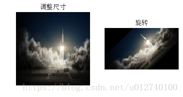
1.2 Matplotlib
可绘制高质量图表,详见:http://matplotlib.sourceforge.net/
1.2.1绘制图像、点和线
from PIL import Image
from pylab import * #在pylab库中,约定图像的左上角为坐标原点

#读取图像到数组中
im = array(Image.open('C:/Users/lbf/Pictures/spaceX.jpg'))

#绘制图像
imshow(im)

#一些点
x = [100,100,400,400]
y = [200,500,200,500] #坐标(100,200),(100,500),(400,200),(400,500)

#使用红色星状标记绘制点
plot(x, y, 'r*')

# 绘制连接前两个点的线
plot(x[:2],y[:2])

# 添加标题,显示绘制图像
title('Plotting')
axis('off') #关闭坐标轴
show()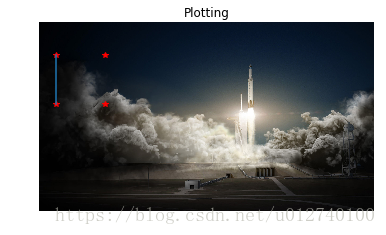
plot(x,y)      #默认为蓝色实线
plot(x,y,'r*')   #红色星状标记
plot(x,y,'go-')  #带有圆圈标记的绿线
plot(x,y,'ks:') #带有正方形标记的黑色点线| 颜色 | 线型 | 标记 | |||
|---|---|---|---|---|---|
| ‘b’ | 蓝色 | ‘-‘ | 实线 | ‘.’ | 点 |
| ‘g’ | 绿色 | ‘–’ | 虚线 | ‘o’ | 圆圈 |
| ‘r’ | 红色 | ‘:’ | 点线 | ’s’ | 正方形 |
| ‘c’ | 青色 | ‘*’ | 星形 | ||
| ‘m’ | 品红 | ‘+’ | 加号 | ||
| ‘y’ | 黄色 | ‘x’ | 叉号 | ||
| ‘k’/’w’ | 黑色/白色 |
1.2.2 图像轮廓和直方图
from PIL import Image
from pylab import *

# 添加中文字体支持
from matplotlib.font_manager import FontProperties
font = FontProperties(fname=r"c:\windows\fonts\SimSun.ttc", size=14)
im = array(Image.open('C:/Users/lbf/Pictures/spaceX.jpg').convert('L'))  # 打开图像,并转成灰度图像

figure() #新建一个图像
subplot(121)
gray()  #不使用颜色信息
contour(im, origin='image')  #在原点的左上角显示轮廓图像
axis('equal')
axis('off')
title(u'图像轮廓', fontproperties=font)

subplot(122)
hist(im.flatten(), 128)  #hist()只接受一维数组作为输入,flatten()方法将任意数组按照行有限准则转换成一维数组
title(u'图像直方图', fontproperties=font)
plt.xlim([0,260])
plt.ylim([0,11000])

show()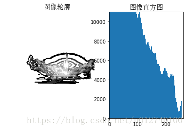
1.2.3交互式标注
#E:/py-works/gin.py
# cmd 中输入 python E:/py-works/gin.py
from PIL import Image
from pylab import *

im = array(Image.open('C:/Users/lbf/Pictures/spaceX.jpg'))
imshow(im)
print ('Please click 3 points')
imshow(im)
x = ginput(3)
print ('You clicked:', x)

show()
1.3Numpy
科学计算工具包,详见:https://docs.scipy.org/doc/numpy/reference/
1.3.1 图像数组表示
from PIL import Image
from pylab import *

im = array(Image.open('C:/Users/lbf/Pictures/spaceX.jpg'))
print (im.shape, im.dtype)
value = im[200, 300, 2]  #访问像素值
print (value)
im = array(Image.open('C:/Users/lbf/Pictures/spaceX.jpg').convert('L'),'f')
print (im.shape, im.dtype)
(1152, 2048, 3) uint8
19
(1152, 2048) float32
多个数组元素可使用数组切片方式访问,如下:
im[i,:] = im[j,:] # 将第j行的数值赋值给第i行
im[:,i] = 100 # 将第i列的所有数值设为500
im[:100,:50].sum() # 计算前100行,前50列所有数值的和
im[i].mean() # 第i行所有数值的平均值
im[:,-1] # 最后一列
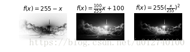
im[-2,:](or im[-2]) #倒数第二行1.3.2 灰度变换
 # -*- coding: utf-8 -*-
from PIL import Image
from numpy import *
from pylab import *

im = array(Image.open('C:/Users/lbf/Pictures/spaceX.jpg').convert('L'))
print (int(im.min()), int(im.max()))

im2 = 255 - im  # invert image反相处理
print (int(im2.min()), int(im2.max()))

im3 = (100.0/255) * im + 100  # clamp to interval 100...200 将图像像素值变换到100-200区间
print (int(im3.min()), int(im3.max()))

im4 = 255.0 * (im/255.0)**2  # squared 对图像像素值求平凡后得到图像
print (int(im4.min()), int(im4.max()))

figure()
gray()
subplot(1, 3, 1)
imshow(im2)
axis('off')
title(r'$f(x)=255-x$')

subplot(1, 3, 2)
imshow(im3)
axis('off')
title(r'$f(x)=\frac{100}{255}x+100$')

subplot(1, 3, 3)
imshow(im4)
axis('off')
title(r'$f(x)=255(\frac{x}{255})^2$')
show()
0 255
0 255
100 200
0 255
# array()变换的相反操作,PIL中的 fromarray() 函数
pil_im = Image.fromarray(im)
pil_im = Image.fromarray(uint8(im))  #设置数据类型
1.3.4直方图均衡化
将一幅图像的灰度直方图扁平,使变换后的图像中每个灰度值的分布概率都相同,是对图像灰度值进行归一化的有效方法,可增强图像对比度。
源码参见:imtool.py 中 histeq()函数
 # -*- coding: utf-8 -*-
from PIL import Image
from pylab import *
from PCV.tools import imtools

# 添加中文字体支持
from matplotlib.font_manager import FontProperties
font = FontProperties(fname=r"c:\windows\fonts\SimSun.ttc", size=14)

im = array(Image.open('C:/Users/lbf/Pictures/ss.jpg').convert('L'))  # 打开图像,并转成灰度图像
#im = array(Image.open('../data/AquaTermi_lowcontrast.JPG').convert('L'))
im2, cdf = imtools.histeq(im)

figure()
subplot(2, 2, 1)
axis('off')
gray()
title(u'原始图像', fontproperties=font)
imshow(im)

subplot(2, 2, 2)
axis('off')
title(u'直方图均衡化后的图像', fontproperties=font)
imshow(im2)

subplot(2, 2, 3)
axis('off')
title(u'原始直方图', fontproperties=font)
#hist(im.flatten(), 128, cumulative=True, normed=True)
hist(im.flatten(), 128, normed=True)

subplot(2, 2, 4)
axis('off')
title(u'均衡化后的直方图', fontproperties=font)
#hist(im2.flatten(), 128, cumulative=True, normed=True)
hist(im2.flatten(), 128, normed=True)

show()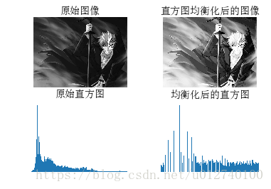
1.3.5图像平均
减少图像噪声的一种简单方式,通常用于艺术特效,图像须有相同尺寸。源码参见:imtool.py 中 compute_average()函数
# -*- coding: utf-8 -*-
from PCV.tools.imtools import get_imlist
from PIL import Image
from pylab import *
from PCV.tools import imtools

# 添加中文字体支持
from matplotlib.font_manager import FontProperties
font = FontProperties(fname=r"c:\windows\fonts\SimSun.ttc", size=14)

filelist = get_imlist('C:/Users/lbf/Pictures/avg/') #获取convert_images_format_test文件夹下的图片文件名(包括后缀名)
avg = imtools.compute_average(filelist)

for impath in filelist:
        im1 = array(Image.open(impath))
        subplot(2, 2, filelist.index(impath)+1)
        imshow(im1)
        imNum=str(filelist.index(impath)+1)
        title(u'待平均图像'+imNum, fontproperties=font)
        axis('off')
subplot(2, 2, 4)
imshow(avg)
title(u'平均后的图像', fontproperties=font)
axis('off')

show()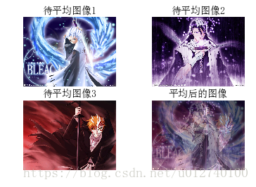
1.3.6 主成分分析(PCA)
PCA(Principal Component Analysis)是一种有用的降维技巧。它可以在使用尽可能少维数的前提下,尽量多地保持训练数据的信息。
(这块单独学习)
1.3.7 使用pickle模块
用于保存一些结果或数据以方便后续使用。pickle模块可以接受几乎所有的python对象,并将其转换成字符串表示,该过程叫做封装(pickling).从字符串表示中重构该对象,成为拆封(unpickling),这些字符串表示可以方便地存储和传输。
1.4 SciPy
SciPy(http://scipy.org/) 是一个开源的数学工具包,它是建立在NumPy的基础上的。它提供了很多有效的常规操作,包括数值综合、最优化、统计、信号处理以及图像处理。
1.4.1 图像模糊
一个经典的并且十分有用的图像卷积例子是对图像进行高斯模糊。高斯模糊可以用于定义图像尺度、计算兴趣点以及很多其他的应用场合。
图像模糊就是将(灰度)图像
I
I
和一个高斯核进行卷积操作:,其中
∗
∗
表示卷积操作;是标准差为
σ
σ
的二维高斯核,定义为
Gσ=12πσ2e−(x2+y2)/2σ2
G
σ
=
1
2
π
σ
2
e
−
(
x
2
+
y
2
)
/
2
σ
2
。
from PIL import Image
from pylab import *
from scipy.ndimage import filters  #滤波操作模块

# 添加中文字体支持
from matplotlib.font_manager import FontProperties
font = FontProperties(fname=r"c:\windows\fonts\SimSun.ttc", size=14)

#im = array(Image.open('board.jpeg'))
im = array(Image.open('C:/Users/lbf/Pictures/spaceX.jpg').convert('L'))

figure()
gray()
axis('off')
subplot(1, 4, 1)
axis('off')
title(u'原图', fontproperties=font)
imshow(im)

for bi, blur in enumerate([2, 5, 10]):  #enumerate参数是一个迭代器对象,比如可以是列表,字符串等,输出索引值和对应的元素值 bi=0,1,2
  im2 = zeros(im.shape)
  im2 = filters.gaussian_filter(im, blur)  #高斯滤波,blur为标注差,分别为2,5,10
  im2 = np.uint8(im2)
  imNum=str(blur)
  subplot(1, 4, 2 + bi)
  axis('off')
  title(u'标准差为'+imNum, fontproperties=font)
  imshow(im2)

#如果是彩色图像,则分别对三个通道进行模糊
#for bi, blur in enumerate([2, 5, 10]):
#  im2 = zeros(im.shape)
#  for i in range(3):
#    im2[:, :, i] = filters.gaussian_filter(im[:, :, i], blur)
#  im2 = np.uint8(im2)
#  subplot(1, 4,  2 + bi)
#  axis('off')
#  imshow(im2)

show()
1.4.2 图像导数
记录强度变化信息。对2-D图像:梯度向量为
∇I=[Ix,Iy]
∇
I
=
[
I
x
,
I
y
]
,梯度大小(描述图像变化强弱):
|∇I|=I2x+I2y−−−−−−√
|
∇
I
|
=
I
x
2
+
I
y
2
,梯度角度(描述图像中每个像素上强度变化的最大方向):
α=arctan2(Iy,Ix)
α
=
a
r
c
t
a
n
2
(
I
y
,
I
x
)
。
用离散近似的方式来计算图像的导数,图像的导数大多数可以通过卷积简单地实现:
Ix=I∗Dx,Iy=I∗Dy
I
x
=
I
∗
D
x
,
I
y
=
I
∗
D
y
,对于
Dx,Dy
D
x
,
D
y
,通常选用Prewitt滤波器:
或Sobel滤波器:
正导数显示为亮的像素,负导数显示为暗的像素,灰色区域表示导数的值接近0。
from PIL import Image
from pylab import *
from scipy.ndimage import filters
import numpy

# 添加中文字体支持
from matplotlib.font_manager import FontProperties
font = FontProperties(fname=r"c:\windows\fonts\SimSun.ttc", size=14)

im = array(Image.open('C:/Users/lbf/Pictures/spaceX.jpg').convert('L'))
gray()

subplot(1, 4, 1)
axis('off')
title(u'(a)原图', fontproperties=font)
imshow(im)

# Sobel derivative filters
imx = zeros(im.shape)
filters.sobel(im, 1, imx)
subplot(1, 4, 2)
axis('off')
title(u'(b)x方向差分', fontproperties=font)
imshow(imx)

imy = zeros(im.shape)
filters.sobel(im, 0, imy)
subplot(1, 4, 3)
axis('off')
title(u'(c)y方向差分', fontproperties=font)
imshow(imy)

#mag = numpy.sqrt(imx**2 + imy**2)
mag = 255-numpy.sqrt(imx**2 + imy**2)
subplot(1, 4, 4)
title(u'(d)梯度幅度', fontproperties=font)
axis('off')
imshow(mag)

show()
#使用高斯导数滤波器
from PIL import Image
from pylab import *
from scipy.ndimage import filters
import numpy

def imx(im, sigma):  #x方向
    imgx = zeros(im.shape)
    filters.gaussian_filter(im, sigma, (0, 1), imgx)
    return imgx

def imy(im, sigma):  #y方向
    imgy = zeros(im.shape)
    filters.gaussian_filter(im, sigma, (1, 0), imgy)
    return imgy

def mag(im, sigma):  #x+y
    # there's also gaussian_gradient_magnitude()
    #mag = numpy.sqrt(imgx**2 + imgy**2)
    imgmag = 255 - numpy.sqrt(imgx ** 2 + imgy ** 2)
    return imgmag

im = array(Image.open('C:/Users/lbf/Pictures/spaceX.jpg').convert('L'))
figure()
gray()

sigma = [2, 5, 10]

for i in  sigma:
    subplot(3, 4, 4*(sigma.index(i))+1)
    axis('off')
    imshow(im)
    imgx=imx(im, i)
    subplot(3, 4, 4*(sigma.index(i))+2)
    axis('off')
    imshow(imgx)
    imgy=imy(im, i)
    subplot(3, 4, 4*(sigma.index(i))+3)
    axis('off')
    imshow(imgy)
    imgmag=mag(im, i)
    subplot(3, 4, 4*(sigma.index(i))+4)
    axis('off')
    imshow(imgmag)

show()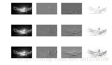
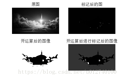
1.4.3 形态学:对象计数
形态学(或数学形态学)是度量和分析基本形状的图像处理方法的基本框架与集合。常用于二值图像,不过它也可以用于灰度图像。二值图像像素只有两种取值,通常是0和1。二值图像通常是由一幅图像进行二值化处理后的产生的,它可以用于用于对物体进行计数,或计算它们的大小。对形态学的介绍和较好的介绍是Mathematical morphology。
from PIL import Image
from numpy import *
from scipy.ndimage import measurements, morphology  #measurements模块实现二值图像的计数和度量功能,morphology模块实现形态学操作。
from pylab import *

"""   This is the morphology counting objects example in Section 1.4.  """

# 添加中文字体支持
from matplotlib.font_manager import FontProperties
font = FontProperties(fname=r"c:\windows\fonts\SimSun.ttc", size=14)

# load image and threshold to make sure it is binary
figure()
gray()
im = array(Image.open('C:/Users/lbf/Pictures/spaceX.jpg').convert('L'))
subplot(221)
imshow(im)
axis('off')
title(u'原图', fontproperties=font)
im = (im < 128)

labels, nbr_objects = measurements.label(im)  #图像的灰度值表示对象的标签
print ("Number of objects:", nbr_objects)
subplot(222)
imshow(labels)
axis('off')
title(u'标记后的图', fontproperties=font)

# morphology - opening to separate objects better
im_open = morphology.binary_opening(im, ones((9, 5)), iterations=4)  #开操作,第二个参数为结构元素,iterations觉定执行该操作的次数
subplot(223)
imshow(im_open)
axis('off')
title(u'开运算后的图像', fontproperties=font)

labels_open, nbr_objects_open = measurements.label(im_open)
print ("Number of objects:", nbr_objects_open)
subplot(224)
imshow(labels_open)
axis('off')
title(u'开运算后进行标记后的图像', fontproperties=font)

show()
Number of objects: 229
Number of objects: 5
1.4.4 有用的SciPy模块
SciPy有一些用于输入和输出数据有用的模块,其中两个是io和misc。
1.读写.mat文件
data = scipy.io.loadmat('test.mat')如果要保存到.mat文件中的话,同样也很容易,仅仅只需要创建一个字典,字典中即可保存你想保存的所有变量,然后用savemat()方法即可:
#创建字典
data = {}
#将变量x保存在字典中
data['x'] = x
scipy.io.savemat('test.mat',data)
更多关于scipy.io的信息可以参阅在线文档[docs.scipy.org/doc/scipy/reference/io.html]。
2.以图像形式保存数组
在scipy.misc模块中,包含了imsave()函数,要保存数组为一幅图像,可通过下面方式完成:
from scipy.misc import imsave
imsave('test.jpg',im)
1.5 更高级的例子:图像降噪
图像降噪是一个在尽可能保持图像细节和结构信息时去除噪声的过程。我们采用Rudin-Osher-Fatemi de-noising(ROF)模型。该模型使处理后的图像更平滑,同时保持图像边缘和结构信息。
一幅灰度图像
I
I
的全变差(Total Variation, TV)定义为梯度范数之和,离散情况下表示为:
ROF模型,目标函数为寻找降噪后的图像
U
U
,使下式最小:,范数
||I−U||
|
|
I
−
U
|
|
是去噪后图像
U
U
和原始图像差异的度量。
from pylab import *
from numpy import *
from numpy import random
from scipy.ndimage import filters
from scipy.misc import imsave
from PCV.tools import rof

""" This is the de-noising example using ROF in Section 1.5. """

# 添加中文字体支持
from matplotlib.font_manager import FontProperties
font = FontProperties(fname=r"c:\windows\fonts\SimSun.ttc", size=14)

# create synthetic image with noise
im = zeros((500,500))
im[100:400,100:400] = 128
im[200:300,200:300] = 255
im = im + 30*random.standard_normal((500,500))

U,T = rof.denoise(im,im)  #roll()函数:循环滚动数组中的元素,计算领域元素的差异。linalg.norm()函数可以衡量两个数组见得差异。
G = filters.gaussian_filter(im,10)


# save the result
#imsave('synth_original.pdf',im)
#imsave('synth_rof.pdf',U)
#imsave('synth_gaussian.pdf',G)


# plot
figure()
gray()

subplot(1,3,1)
imshow(im)
#axis('equal')
axis('off')
title(u'原噪声图像', fontproperties=font)

subplot(1,3,2)
imshow(G)
#axis('equal')
axis('off')
title(u'高斯模糊后的图像', fontproperties=font)

subplot(1,3,3)
imshow(U)
#axis('equal')
axis('off')
title(u'ROF降噪后的图像', fontproperties=font)

show()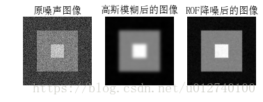


 1628
1628


 被折叠的 条评论
为什么被折叠?
被折叠的 条评论
为什么被折叠?
 到【灌水乐园】发言


