


写在前面
博主前期科研工作中,涉及到要对某个地区的一些空间点进行聚类分析,想到读研期间,曾经用DBSCAN聚类算法实现了四线激光雷达扫描的三维点云数据聚类(论文题目:基于改进DBSCAN算法的激光雷达目标物检测方法),当初用matlab实现的,虽说是改进的算法,但改进方法非常原始。DBSCAN是一种非常实用的密度聚类算法,而地理空间的经纬度点聚类,没有其他维度的信息的话,毫无疑问可以用密度聚类。于是博主重新熟悉了一下算法,并做了一些改进,用Python实现,记录在博客里面。
- 编译环境:Python3.7
- 编译器:Spyder 4.1.5
算法及实现过程
DBSCAN聚类算法原理
先简单介绍一下DBSCAN聚类算法的原理:
DBSCAN(Density-based spatial clustering of applications with noise)是由Martin Ester[8]等人最早提出的一种基于密度的空间聚类算法,该算法将具有足够密度数据的区域划分为k个不同的簇,并能在具有噪声数据的空间域内发现任意形状的簇,本文记为Cj(j=1,2…k),其中簇定义为密度相连点的最大集合,其基本原理是聚类过程要满足以下两个条件:最大性,对于空间中任意两点p、q,如果p属于簇C,并且p密度可达q,则点q也属于簇C;连接性,对于同属于簇的任意两点p、q,它们彼此是密度相连的。DBSCAN算法具有聚类速度快、能有效处理噪声点、能发现空间中任意形状簇、无需划分聚类个数等优点,但DBSCAN聚类算法也有其缺点,其聚类效果高度依赖输入参数——聚类半径和簇内最少样本点数,在高维数据的聚类中,对距离公式选取非常敏感,存在“维数灾难”。
上面一段引自自己的论文,很不好理解对不对,博主也不打算花精力去解释,因为单独理解这个聚类算法,估计都得写篇博客。想理解原理的,自己在CSDN里面搜,能搜出一大堆博客来,给大家推荐一篇博客,看完基本就明白了。
DBSCAN聚类算法——机器学习(理论+图解+python代码)
简单来说,DBSCAN聚类算法需要有数据点,最好是三维以内,高维数据聚类很复杂;需要一个聚类半径,按照核心点搜索半径邻域内的其他点;需要一个聚类最少点数,也就是一个类里面,最少要包含特定数量的点。
Python实现原始的DBSCAN聚类算法
DBSCAN聚类算法是机器学习的一种,说到用Python做机器学习,那自然少不了sklearn这个包,这个包里面有cluster方法是专门用来聚类的,而这个聚类函数里面,又有个DBSCAN类,我们来看看这个类吧(为了不影响阅读体验,我建议大家直接跳过不要看,太长了)
# -*- coding: utf-8 -*-
"""
DBSCAN: Density-Based Spatial Clustering of Applications with Noise
"""

# Author: Robert Layton <robertlayton@gmail.com>
#         Joel Nothman <joel.nothman@gmail.com>
#         Lars Buitinck
#
# License: BSD 3 clause

import numpy as np
import warnings
from scipy import sparse

from ..base import BaseEstimator, ClusterMixin
from ..utils.validation import _check_sample_weight, _deprecate_positional_args
from ..neighbors import NearestNeighbors

from ._dbscan_inner import dbscan_inner


@_deprecate_positional_args
def dbscan(X, eps=0.5, *, min_samples=5, metric='minkowski',
           metric_params=None, algorithm='auto', leaf_size=30, p=2,
           sample_weight=None, n_jobs=None):
    """Perform DBSCAN clustering from vector array or distance matrix.

    Read more in the :ref:`User Guide <dbscan>`.

    Parameters
    ----------
    X : {array-like, sparse (CSR) matrix} of shape (n_samples, n_features) or \
            (n_samples, n_samples)
        A feature array, or array of distances between samples if
        ``metric='precomputed'``.

    eps : float, default=0.5
        The maximum distance between two samples for one to be considered
        as in the neighborhood of the other. This is not a maximum bound
        on the distances of points within a cluster. This is the most
        important DBSCAN parameter to choose appropriately for your data set
        and distance function.

    min_samples : int, default=5
        The number of samples (or total weight) in a neighborhood for a point
        to be considered as a core point. This includes the point itself.

    metric : string, or callable
        The metric to use when calculating distance between instances in a
        feature array. If metric is a string or callable, it must be one of
        the options allowed by :func:`sklearn.metrics.pairwise_distances` for
        its metric parameter.
        If metric is "precomputed", X is assumed to be a distance matrix and
        must be square during fit.
        X may be a :term:`sparse graph <sparse graph>`,
        in which case only "nonzero" elements may be considered neighbors.

    metric_params : dict, default=None
        Additional keyword arguments for the metric function.

        .. versionadded:: 0.19

    algorithm : {'auto', 'ball_tree', 'kd_tree', 'brute'}, default='auto'
        The algorithm to be used by the NearestNeighbors module
        to compute pointwise distances and find nearest neighbors.
        See NearestNeighbors module documentation for details.

    leaf_size : int, default=30
        Leaf size passed to BallTree or cKDTree. This can affect the speed
        of the construction and query, as well as the memory required
        to store the tree. The optimal value depends
        on the nature of the problem.

    p : float, default=2
        The power of the Minkowski metric to be used to calculate distance
        between points.

    sample_weight : array-like of shape (n_samples,), default=None
        Weight of each sample, such that a sample with a weight of at least
        ``min_samples`` is by itself a core sample; a sample with negative
        weight may inhibit its eps-neighbor from being core.
        Note that weights are absolute, and default to 1.

    n_jobs : int, default=None
        The number of parallel jobs to run for neighbors search. ``None`` means
        1 unless in a :obj:`joblib.parallel_backend` context. ``-1`` means
        using all processors. See :term:`Glossary <n_jobs>` for more details.
        If precomputed distance are used, parallel execution is not available
        and thus n_jobs will have no effect.

    Returns
    -------
    core_samples : ndarray of shape (n_core_samples,)
        Indices of core samples.

    labels : ndarray of shape (n_samples,)
        Cluster labels for each point.  Noisy samples are given the label -1.

    See also
    --------
    DBSCAN
        An estimator interface for this clustering algorithm.
    OPTICS
        A similar estimator interface clustering at multiple values of eps. Our
        implementation is optimized for memory usage.

    Notes
    -----
    For an example, see :ref:`examples/cluster/plot_dbscan.py
    <sphx_glr_auto_examples_cluster_plot_dbscan.py>`.

    This implementation bulk-computes all neighborhood queries, which increases
    the memory complexity to O(n.d) where d is the average number of neighbors,
    while original DBSCAN had memory complexity O(n). It may attract a higher
    memory complexity when querying these nearest neighborhoods, depending
    on the ``algorithm``.

    One way to avoid the query complexity is to pre-compute sparse
    neighborhoods in chunks using
    :func:`NearestNeighbors.radius_neighbors_graph
    <sklearn.neighbors.NearestNeighbors.radius_neighbors_graph>` with
    ``mode='distance'``, then using ``metric='precomputed'`` here.

    Another way to reduce memory and computation time is to remove
    (near-)duplicate points and use ``sample_weight`` instead.

    :func:`cluster.optics <sklearn.cluster.optics>` provides a similar
    clustering with lower memory usage.

    References
    ----------
    Ester, M., H. P. Kriegel, J. Sander, and X. Xu, "A Density-Based
    Algorithm for Discovering Clusters in Large Spatial Databases with Noise".
    In: Proceedings of the 2nd International Conference on Knowledge Discovery
    and Data Mining, Portland, OR, AAAI Press, pp. 226-231. 1996

    Schubert, E., Sander, J., Ester, M., Kriegel, H. P., & Xu, X. (2017).
    DBSCAN revisited, revisited: why and how you should (still) use DBSCAN.
    ACM Transactions on Database Systems (TODS), 42(3), 19.
    """

    est = DBSCAN(eps=eps, min_samples=min_samples, metric=metric,
                 metric_params=metric_params, algorithm=algorithm,
                 leaf_size=leaf_size, p=p, n_jobs=n_jobs)
    est.fit(X, sample_weight=sample_weight)
    return est.core_sample_indices_, est.labels_


class DBSCAN(ClusterMixin, BaseEstimator):
    """Perform DBSCAN clustering from vector array or distance matrix.

    DBSCAN - Density-Based Spatial Clustering of Applications with Noise.
    Finds core samples of high density and expands clusters from them.
    Good for data which contains clusters of similar density.

    Read more in the :ref:`User Guide <dbscan>`.

    Parameters
    ----------
    eps : float, default=0.5
        The maximum distance between two samples for one to be considered
        as in the neighborhood of the other. This is not a maximum bound
        on the distances of points within a cluster. This is the most
        important DBSCAN parameter to choose appropriately for your data set
        and distance function.

    min_samples : int, default=5
        The number of samples (or total weight) in a neighborhood for a point
        to be considered as a core point. This includes the point itself.

    metric : string, or callable, default='euclidean'
        The metric to use when calculating distance between instances in a
        feature array. If metric is a string or callable, it must be one of
        the options allowed by :func:`sklearn.metrics.pairwise_distances` for
        its metric parameter.
        If metric is "precomputed", X is assumed to be a distance matrix and
        must be square. X may be a :term:`Glossary <sparse graph>`, in which
        case only "nonzero" elements may be considered neighbors for DBSCAN.

        .. versionadded:: 0.17
           metric *precomputed* to accept precomputed sparse matrix.

    metric_params : dict, default=None
        Additional keyword arguments for the metric function.

        .. versionadded:: 0.19

    algorithm : {'auto', 'ball_tree', 'kd_tree', 'brute'}, default='auto'
        The algorithm to be used by the NearestNeighbors module
        to compute pointwise distances and find nearest neighbors.
        See NearestNeighbors module documentation for details.

    leaf_size : int, default=30
        Leaf size passed to BallTree or cKDTree. This can affect the speed
        of the construction and query, as well as the memory required
        to store the tree. The optimal value depends
        on the nature of the problem.

    p : float, default=None
        The power of the Minkowski metric to be used to calculate distance
        between points.

    n_jobs : int, default=None
        The number of parallel jobs to run.
        ``None`` means 1 unless in a :obj:`joblib.parallel_backend` context.
        ``-1`` means using all processors. See :term:`Glossary <n_jobs>`
        for more details.

    Attributes
    ----------
    core_sample_indices_ : ndarray of shape (n_core_samples,)
        Indices of core samples.

    components_ : ndarray of shape (n_core_samples, n_features)
        Copy of each core sample found by training.

    labels_ : ndarray of shape (n_samples)
        Cluster labels for each point in the dataset given to fit().
        Noisy samples are given the label -1.

    Examples
    --------
    >>> from sklearn.cluster import DBSCAN
    >>> import numpy as np
    >>> X = np.array([[1, 2], [2, 2], [2, 3],
    ...               [8, 7], [8, 8], [25, 80]])
    >>> clustering = DBSCAN(eps=3, min_samples=2).fit(X)
    >>> clustering.labels_
    array([ 0,  0,  0,  1,  1, -1])
    >>> clustering
    DBSCAN(eps=3, min_samples=2)

    See also
    --------
    OPTICS
        A similar clustering at multiple values of eps. Our implementation
        is optimized for memory usage.

    Notes
    -----
    For an example, see :ref:`examples/cluster/plot_dbscan.py
    <sphx_glr_auto_examples_cluster_plot_dbscan.py>`.

    This implementation bulk-computes all neighborhood queries, which increases
    the memory complexity to O(n.d) where d is the average number of neighbors,
    while original DBSCAN had memory complexity O(n). It may attract a higher
    memory complexity when querying these nearest neighborhoods, depending
    on the ``algorithm``.

    One way to avoid the query complexity is to pre-compute sparse
    neighborhoods in chunks using
    :func:`NearestNeighbors.radius_neighbors_graph
    <sklearn.neighbors.NearestNeighbors.radius_neighbors_graph>` with
    ``mode='distance'``, then using ``metric='precomputed'`` here.

    Another way to reduce memory and computation time is to remove
    (near-)duplicate points and use ``sample_weight`` instead.

    :class:`cluster.OPTICS` provides a similar clustering with lower memory
    usage.

    References
    ----------
    Ester, M., H. P. Kriegel, J. Sander, and X. Xu, "A Density-Based
    Algorithm for Discovering Clusters in Large Spatial Databases with Noise".
    In: Proceedings of the 2nd International Conference on Knowledge Discovery
    and Data Mining, Portland, OR, AAAI Press, pp. 226-231. 1996

    Schubert, E., Sander, J., Ester, M., Kriegel, H. P., & Xu, X. (2017).
    DBSCAN revisited, revisited: why and how you should (still) use DBSCAN.
    ACM Transactions on Database Systems (TODS), 42(3), 19.
    """
    @_deprecate_positional_args
    def __init__(self, eps=0.5, *, min_samples=5, metric='euclidean',
                 metric_params=None, algorithm='auto', leaf_size=30, p=None,
                 n_jobs=None):
        self.eps = eps
        self.min_samples = min_samples
        self.metric = metric
        self.metric_params = metric_params
        self.algorithm = algorithm
        self.leaf_size = leaf_size
        self.p = p
        self.n_jobs = n_jobs

    def fit(self, X, y=None, sample_weight=None):
        """Perform DBSCAN clustering from features, or distance matrix.

        Parameters
        ----------
        X : {array-like, sparse matrix} of shape (n_samples, n_features), or \
            (n_samples, n_samples)
            Training instances to cluster, or distances between instances if
            ``metric='precomputed'``. If a sparse matrix is provided, it will
            be converted into a sparse ``csr_matrix``.

        sample_weight : array-like of shape (n_samples,), default=None
            Weight of each sample, such that a sample with a weight of at least
            ``min_samples`` is by itself a core sample; a sample with a
            negative weight may inhibit its eps-neighbor from being core.
            Note that weights are absolute, and default to 1.

        y : Ignored
            Not used, present here for API consistency by convention.

        Returns
        -------
        self

        """
        X = self._validate_data(X, accept_sparse='csr')

        if not self.eps > 0.0:
            raise ValueError("eps must be positive.")

        if sample_weight is not None:
            sample_weight = _check_sample_weight(sample_weight, X)

        # Calculate neighborhood for all samples. This leaves the original
        # point in, which needs to be considered later (i.e. point i is in the
        # neighborhood of point i. While True, its useless information)
        if self.metric == 'precomputed' and sparse.issparse(X):
            # set the diagonal to explicit values, as a point is its own
            # neighbor
            with warnings.catch_warnings():
                warnings.simplefilter('ignore', sparse.SparseEfficiencyWarning)
                X.setdiag(X.diagonal())  # XXX: modifies X's internals in-place

        neighbors_model = NearestNeighbors(
            radius=self.eps, algorithm=self.algorithm,
            leaf_size=self.leaf_size, metric=self.metric,
            metric_params=self.metric_params, p=self.p, n_jobs=self.n_jobs)
        neighbors_model.fit(X)
        # This has worst case O(n^2) memory complexity
        neighborhoods = neighbors_model.radius_neighbors(X,
                                                         return_distance=False)

        if sample_weight is None:
            n_neighbors = np.array([len(neighbors)
                                    for neighbors in neighborhoods])
        else:
            n_neighbors = np.array([np.sum(sample_weight[neighbors])
                                    for neighbors in neighborhoods])

        # Initially, all samples are noise.
        labels = np.full(X.shape[0], -1, dtype=np.intp)

        # A list of all core samples found.
        core_samples = np.asarray(n_neighbors >= self.min_samples,
                                  dtype=np.uint8)
        dbscan_inner(core_samples, neighborhoods, labels)

        self.core_sample_indices_ = np.where(core_samples)[0]
        self.labels_ = labels

        if len(self.core_sample_indices_):
            # fix for scipy sparse indexing issue
            self.components_ = X[self.core_sample_indices_].copy()
        else:
            # no core samples
            self.components_ = np.empty((0, X.shape[1]))
        return self

    def fit_predict(self, X, y=None, sample_weight=None):
        """Perform DBSCAN clustering from features or distance matrix,
        and return cluster labels.

        Parameters
        ----------
        X : {array-like, sparse matrix} of shape (n_samples, n_features), or \
            (n_samples, n_samples)
            Training instances to cluster, or distances between instances if
            ``metric='precomputed'``. If a sparse matrix is provided, it will
            be converted into a sparse ``csr_matrix``.

        sample_weight : array-like of shape (n_samples,), default=None
            Weight of each sample, such that a sample with a weight of at least
            ``min_samples`` is by itself a core sample; a sample with a
            negative weight may inhibit its eps-neighbor from being core.
            Note that weights are absolute, and default to 1.

        y : Ignored
            Not used, present here for API consistency by convention.

        Returns
        -------
        labels : ndarray of shape (n_samples,)
            Cluster labels. Noisy samples are given the label -1.
        """
        self.fit(X, sample_weight=sample_weight)
        return self.labels_
代码写的很牛逼,但是不建议看,因为我实在是没耐心看完。
那我们就用这个DBSCAN来写个聚类的示例吧,用鸢尾花数据。
先看看数据的基本特征:
import matplotlib.pyplot as plt
import numpy as np
from sklearn.cluster import KMeans
from sklearn import datasets
from  sklearn.cluster import DBSCAN
plt.rcParams['font.sans-serif'] = ['Microsoft YaHei']

iris = datasets.load_iris()
X = iris.data[:, :4]
# 看看数据
plt.scatter(X[:, 0], X[:, 1], c="red", marker='o', label='see')
plt.xlabel('萼片长度')
plt.ylabel('萼片宽度')
plt.legend(loc=2)
plt.show()
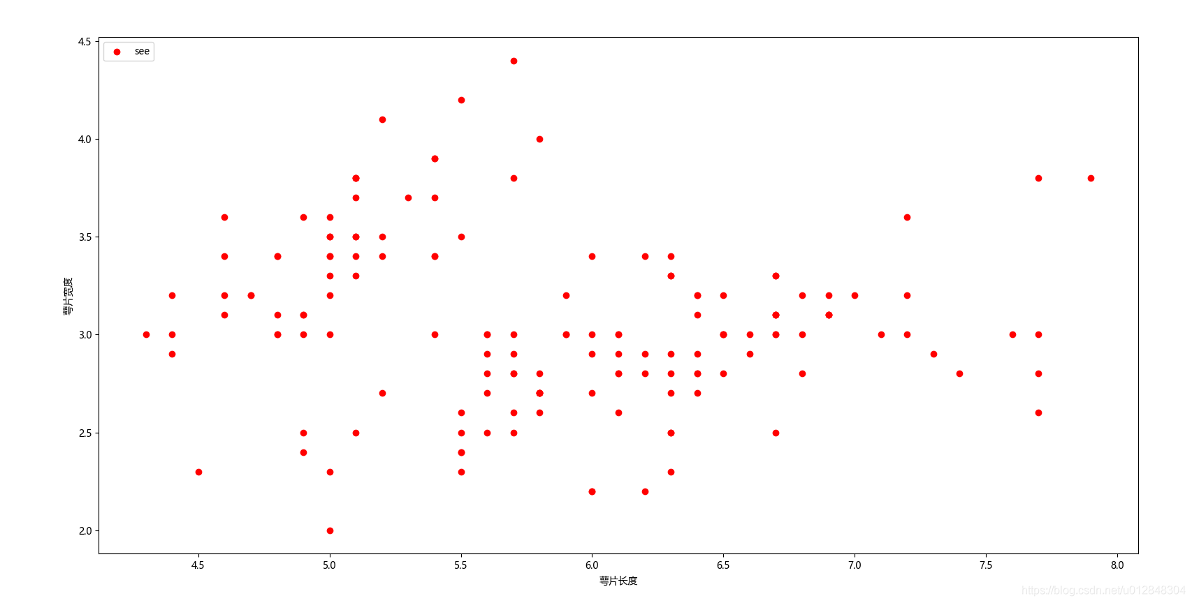
这就是基本的数据分布情况,代码很简单,我不再一一解释。
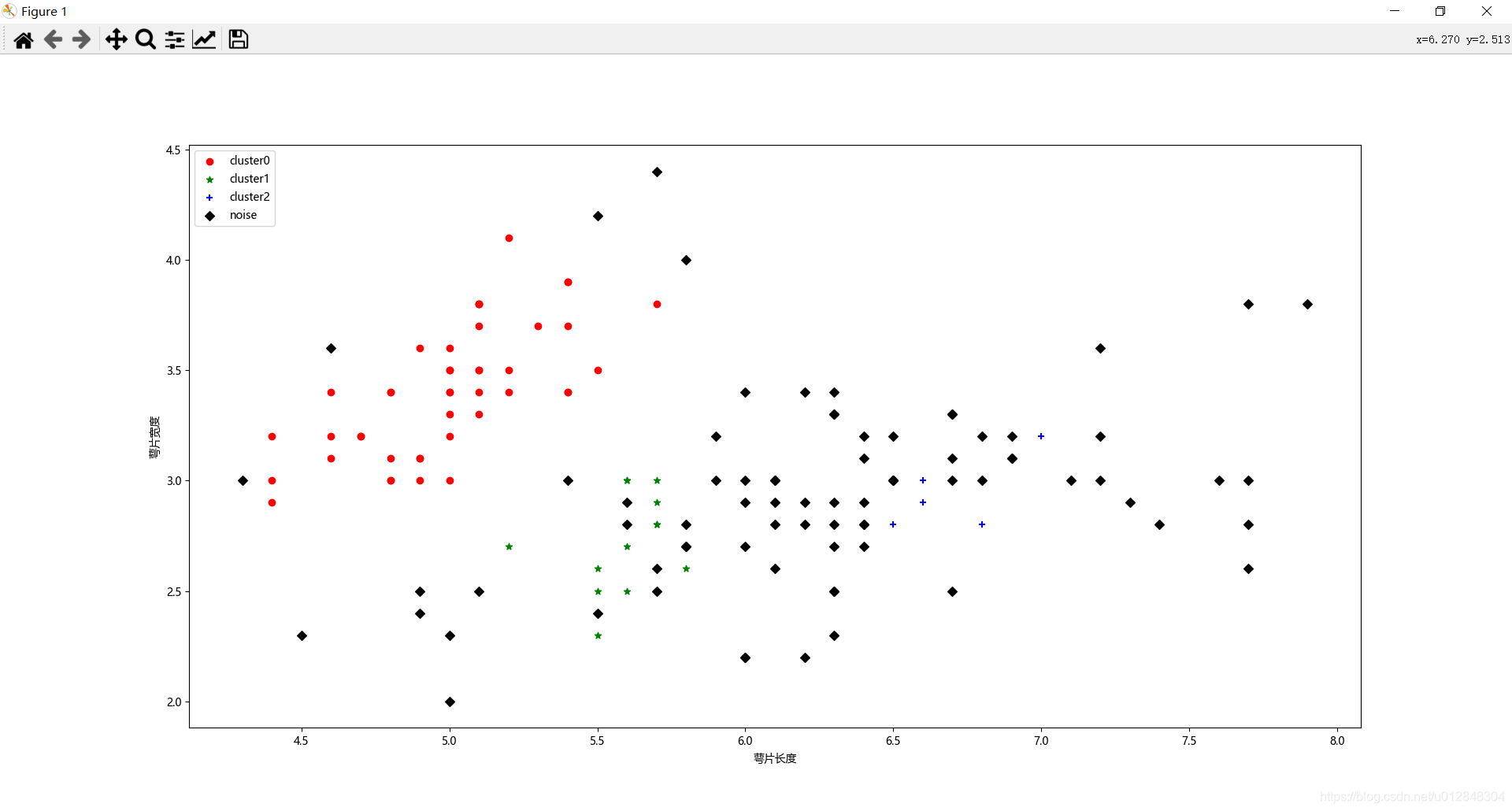
接下来我们看下最原始的DBSCAN聚类算法,直接看代码:
dbscan = DBSCAN(eps=0.4, min_samples=9)  # 1
dbscan.fit(X)   # 2
label_pred = dbscan.labels_  # 3

# 绘制聚类结果
x0 = X[label_pred == 0]  # 4
x1 = X[label_pred == 1]  # 4
x2 = X[label_pred == 2]  # 4
x3 = X[label_pred == -1]   # 4
plt.scatter(x0[:, 0], x0[:, 1], c="red", marker='o', label='cluster0')
plt.scatter(x1[:, 0], x1[:, 1], c="green", marker='*', label='cluster1')
plt.scatter(x2[:, 0], x2[:, 1], c="blue", marker='+', label='cluster2')
plt.scatter(x3[:, 0], x3[:, 1], c="black", marker='D', label='noise')
plt.xlabel('萼片长度')
plt.ylabel('萼片宽度')
plt.legend(loc=2)
plt.show()
我来解释一下我标注的部分:
- dbscan = DBSCAN(eps=0.4, min_samples=9) 表示设置参数,聚类半径是0.4,每个类里面的点不少于9个,也就是我前面说的三个参数中的后两个;
- dbscan.fit(X) 数据集拟合,机器学习无需多言;
- label_pred = dbscan.labels_ 聚类结果,也就是说每个点聚类的情况,如果是-1,说明算法认为这个点是噪声点,我们先来看看聚类结果,如下图(为了方便大家看数据,我把计算得到的label_pred变换了一下,将单列数据变成了6列):
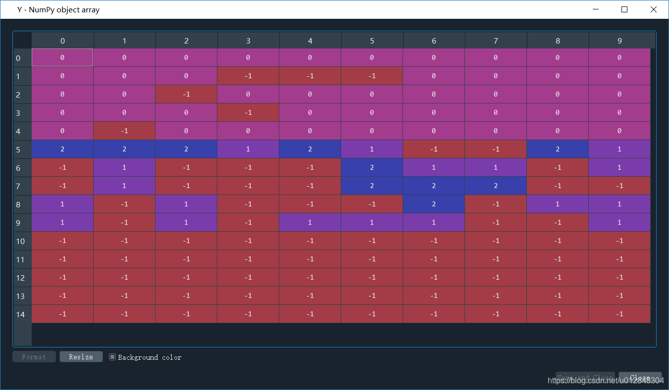
可以看出来,大部分点被归为噪声点,只划分了3个簇,聚类标签分别为0/1/2。 - 后面就是根据聚类的标签值,把数据进行分类,并画出来,来看看聚类结果。
好了,原理就介绍这么多,写了这么多相信大家对DBSCAN聚类算法有了一定的理解,那下面进入我们的正题。
DBSCAN聚类经纬度点
博主手上有一些经纬度数据点,我想用DBSCAN算法来进行聚类。虽然我前面写了,DBSCAN算法的原始代码不建议看,但是关注源代码里面的这一行代码:
def __init__(self, eps=0.5, *, min_samples=5, metric='euclidean',
                 metric_params=None, algorithm='auto', leaf_size=30, p=None, n_jobs=None):
其中有一个关键参数,metric=‘euclidean’,意思就是距离计算公式是欧式距离,但是我们的点集是经纬度数据点,如果直接用欧式距离来表达两个点之间的经纬度距离点,会不会有问题呢?
不管了,先试试看聚类情况。上完整代码
import pandas as pd
import numpy as np
from sklearn.cluster import DBSCAN
import matplotlib.pyplot as plt
import seaborn as sns
import folium
from sklearn import metrics
sns.set()
## 第一部分
df = pd.read_csv('00-首页数据.csv')
df = df[['lat_Amap', 'lng_Amap']].dropna(axis=0,how='all')
data = np.array(df)

db = DBSCAN(eps=0.005, min_samples=10).fit(data)
labels = db.labels_
raito = len(labels[labels[:] == -1]) / len(labels)  # 计算噪声点个数占总数的比例
n_clusters_ = len(set(labels)) - (1 if -1 in labels else 0)  # 获取分簇的数目
score = metrics.silhouette_score(data, labels)

df['label'] = labels
sns.lmplot('lat_Amap', 'lng_Amap', df, hue='label', fit_reg=False)

## 第二部分
map_ = folium.Map(location=[31.574729, 120.301663], zoom_start=12,
                       tiles='http://webrd02.is.autonavi.com/appmaptile?lang=zh_cn&size=1&scale=1&style=7&x={x}&y={y}&z={z}',
                       attr='default')

colors = ['#DC143C', '#FFB6C1', '#DB7093', '#C71585', '#8B008B', '#4B0082', '#7B68EE',
         '#0000FF', '#B0C4DE', '#708090', '#00BFFF', '#5F9EA0', '#00FFFF', '#7FFFAA',
         '#008000', '#FFFF00', '#808000', '#FFD700', '#FFA500', '#FF6347','#DC143C',
         '#FFB6C1', '#DB7093', '#C71585', '#8B008B', '#4B0082', '#7B68EE',
         '#0000FF', '#B0C4DE', '#708090', '#00BFFF', '#5F9EA0', '#00FFFF', '#7FFFAA',
         '#008000', '#FFFF00', '#808000', '#FFD700', '#FFA500', '#FF6347',
         '#DC143C', '#FFB6C1', '#DB7093', '#C71585', '#8B008B', '#4B0082', '#7B68EE',
         '#0000FF', '#B0C4DE', '#708090', '#00BFFF', '#5F9EA0', '#00FFFF', '#7FFFAA',
         '#008000', '#FFFF00', '#808000', '#FFD700', '#FFA500', '#FF6347',
         '#DC143C', '#FFB6C1', '#DB7093', '#C71585', '#8B008B', '#4B0082', '#7B68EE',
         '#0000FF', '#B0C4DE', '#708090', '#00BFFF', '#5F9EA0', '#00FFFF', '#7FFFAA',
         '#008000', '#FFFF00', '#808000', '#FFD700', '#FFA500', '#FF6347','#DC143C',
         '#FFB6C1', '#DB7093', '#C71585', '#8B008B', '#4B0082', '#7B68EE',
         '#0000FF', '#B0C4DE', '#708090', '#00BFFF', '#5F9EA0', '#00FFFF', '#7FFFAA',
         '#008000', '#FFFF00', '#808000', '#FFD700', '#FFA500', '#FF6347',
         '#DC143C', '#FFB6C1', '#DB7093', '#C71585', '#8B008B', '#4B0082', '#7B68EE',
         '#0000FF', '#B0C4DE', '#708090', '#00BFFF', '#5F9EA0', '#00FFFF', '#7FFFAA',
         '#008000', '#FFFF00', '#808000', '#FFD700', '#FFA500', '#FF6347','#000000']

for i in range(len(data)):
    folium.CircleMarker(location=[data[i][0], data[i][1]],
                        radius=4, popup='popup',
                        color=colors[labels[i]], fill=True,
                        fill_color=colors[labels[i]]).add_to(map_)

map_.save('all_cluster.html')
代码很长,我们分两部分来看
第一部分是原始聚类,还有看聚类结果,直接看看sns.lmplot(‘lat_Amap’, ‘lng_Amap’, df, hue=‘label’, fit_reg=False)的效果吧

聚成了40多个类,噪声占比79%。。
感觉还可以接受啊,但是同学们看懂了的话,肯定会有一个疑问:
db = DBSCAN(eps=0.005, min_samples=10).fit(data)
这行代码里面,这两个关键参数是怎么获取的?
比较尴尬,我只能告诉大家,我是一个个试出来,对比原始数据,感觉这个参数最好。
df['label'] = labels
上面这行代码,是将聚类标签加入到原始数组里面去,看看df
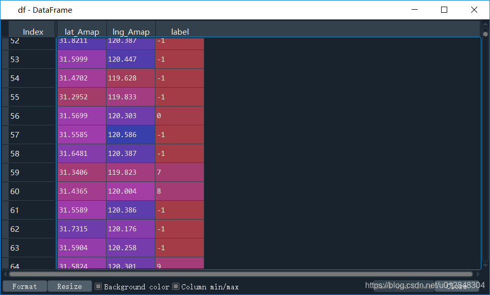
反正有40+类,对于一个市的数据来说,博主觉得研究内容还算合理。
第二部分在干嘛呢,那是博主在将聚类结果打在地图上,用到了folium这个包,这个包很好用,建议看一下我前一篇博客。
当然,我也是根据聚类的标签来画点的颜色的,因此,我定义了40多个颜色,当然,里面是有重复的颜色,不过不影响视觉效果。为了把每个点都用对应的颜色,我写了个循环,看下面的代码:
for i in range(len(data)):
    folium.CircleMarker(location=[data[i][0], data[i][1]],
                        radius=4, popup='popup',
                        color=colors[labels[i]], fill=True,
                        fill_color=colors[labels[i]]).add_to(map_)
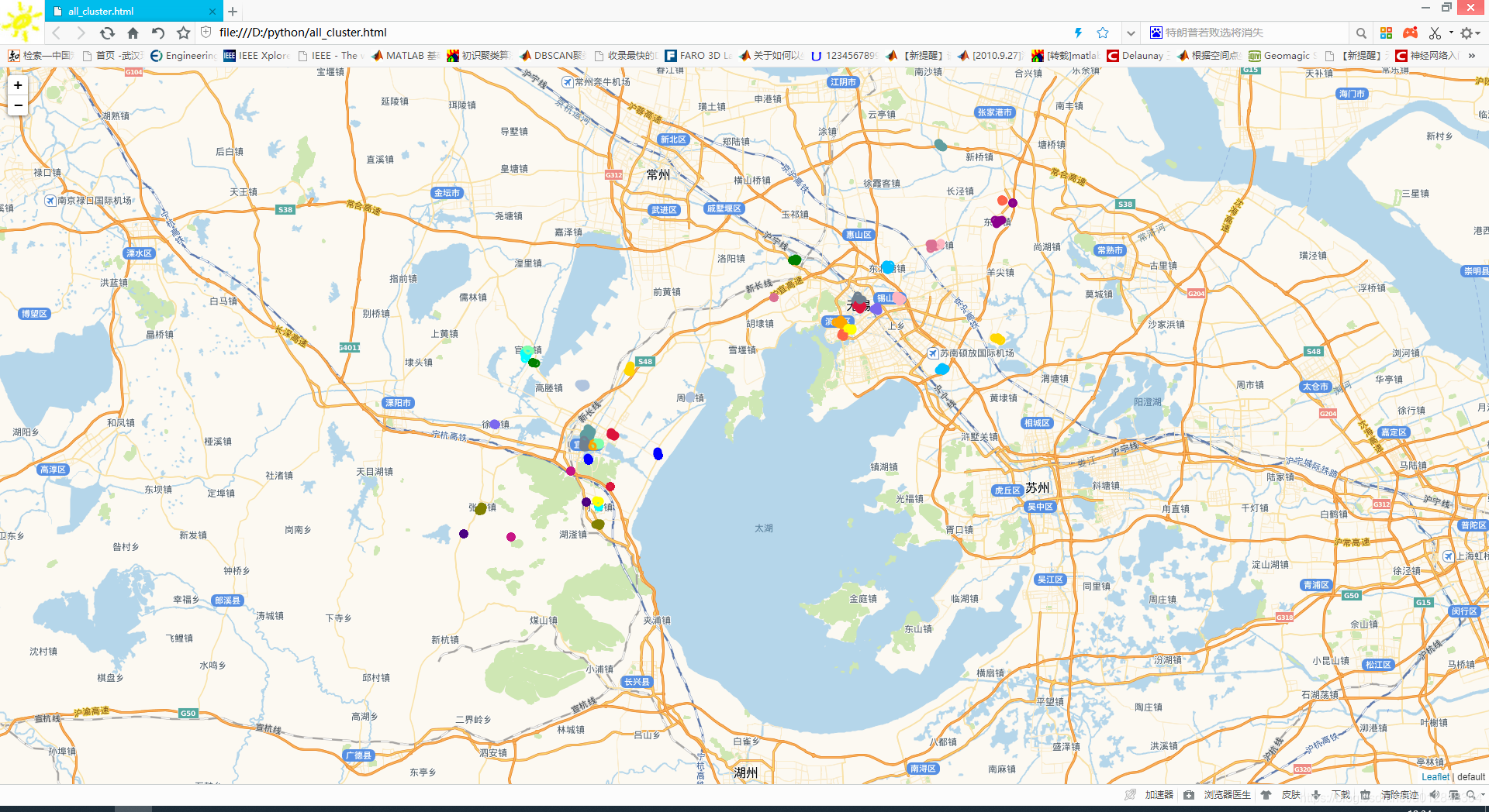
循环是最简单的方法,看地图上的效果
上图中,黑色的圆圈点是噪声点,其他颜色是不同的类。效果还不错,与实际情况一致,也就是说,用欧式距离是可以的,但是博主一直觉得这样做不妥,在网上搜索了很多资料,终于找到方法替换欧式距离了。
经纬度实际距离替换欧式距离并进行聚类
不磨叽,直接上代码
# -*- coding: utf-8 -*-
"""
Created on Fri Jun 12 10:39:07 2020

@author: HP
"""

# -*- coding: utf-8 -*-
"""
Created on Wed May 20 08:32:01 2020

@author: HP
"""

import pandas as pd
import numpy as np
from sklearn.cluster import DBSCAN
import matplotlib.pyplot as plt
import seaborn as sns
import folium
from sklearn import metrics
from  math import radians
from math import tan,atan,acos,sin,cos,asin,sqrt
from scipy.spatial.distance import pdist, squareform
sns.set()

def haversine(lonlat1, lonlat2):
    lat1, lon1 = lonlat1
    lat2, lon2 = lonlat2
    lon1, lat1, lon2, lat2 = map(radians, [lon1, lat1, lon2, lat2])

    dlon = lon2 - lon1
    dlat = lat2 - lat1
    a = sin(dlat / 2) ** 2 + cos(lat1) * cos(lat2) * sin(dlon / 2) ** 2
    c = 2 * asin(sqrt(a))
    r = 6371  # Radius of earth in kilometers. Use 3956 for miles
    return c * r * 1000


df = pd.read_csv('00-首页数据.csv')

df = df[['lat_Amap', 'lng_Amap']].dropna(axis=0,how='all')
# df['lon_lat'] = df.apply(lambda x: [x['lng_Amap'], x['lat_Amap']], axis=1)
# df = df['lon_lat'].to_frame()
# data = np.array(data)
# plt.figure(figsize=(10, 10))
# plt.scatter(df['lat_Amap'], df['lng_Amap'])
distance_matrix = squareform(pdist(df, (lambda u, v: haversine(u, v))))
db = DBSCAN(eps=500, min_samples=10, metric='precomputed').fit_predict(distance_matrix)


'''
db = DBSCAN(eps=0.038, min_samples=3).fit(data)
'''
labels = db
raito = len(labels[labels[:] == -1]) / len(labels)  # 计算噪声点个数占总数的比例
n_clusters_ = len(set(labels)) - (1 if -1 in labels else 0)  # 获取分簇的数目
# score = metrics.silhouette_score(distance_matrix, labels)
df['label'] = labels
sns.lmplot('lat_Amap', 'lng_Amap', df, hue='label', fit_reg=False)

'''
df['label'] = labels
sns.lmplot('lat_Amap', 'lng_Amap', df, hue='label', fit_reg=False)
'''
map_all = folium.Map(location=[31.574729, 120.301663], zoom_start=12,
                     tiles='http://webrd02.is.autonavi.com/appmaptile?lang=zh_cn&size=1&scale=1&style=7&x={x}&y={y}&z={z}',
                     attr='default')

# colors = ['#DC143C', '#FFB6C1', '#DB7093', '#C71585', '#8B008B', '#4B0082', '#7B68EE',
#          '#0000FF', '#B0C4DE', '#708090', '#00BFFF', '#5F9EA0', '#00FFFF', '#7FFFAA',
#          '#008000', '#FFFF00', '#808000', '#FFD700', '#FFA500', '#FF6347', '#000000']

colors = ['#DC143C', '#FFB6C1', '#DB7093', '#C71585', '#8B008B', '#4B0082', '#7B68EE',
         '#0000FF', '#B0C4DE', '#708090', '#00BFFF', '#5F9EA0', '#00FFFF', '#7FFFAA',
         '#008000', '#FFFF00', '#808000', '#FFD700', '#FFA500', '#FF6347','#DC143C',
         '#FFB6C1', '#DB7093', '#C71585', '#8B008B', '#4B0082', '#7B68EE',
         '#0000FF', '#B0C4DE', '#708090', '#00BFFF', '#5F9EA0', '#00FFFF', '#7FFFAA',
         '#008000', '#FFFF00', '#808000', '#FFD700', '#FFA500', '#FF6347',
         '#DC143C', '#FFB6C1', '#DB7093', '#C71585', '#8B008B', '#4B0082', '#7B68EE',
         '#0000FF', '#B0C4DE', '#708090', '#00BFFF', '#5F9EA0', '#00FFFF', '#7FFFAA',
         '#008000', '#FFFF00', '#808000', '#FFD700', '#FFA500', '#FF6347',
         '#DC143C', '#FFB6C1', '#DB7093', '#C71585', '#8B008B', '#4B0082', '#7B68EE',
         '#0000FF', '#B0C4DE', '#708090', '#00BFFF', '#5F9EA0', '#00FFFF', '#7FFFAA',
         '#008000', '#FFFF00', '#808000', '#FFD700', '#FFA500', '#FF6347','#DC143C',
         '#FFB6C1', '#DB7093', '#C71585', '#8B008B', '#4B0082', '#7B68EE',
         '#0000FF', '#B0C4DE', '#708090', '#00BFFF', '#5F9EA0', '#00FFFF', '#7FFFAA',
         '#008000', '#FFFF00', '#808000', '#FFD700', '#FFA500', '#FF6347',
         '#DC143C', '#FFB6C1', '#DB7093', '#C71585', '#8B008B', '#4B0082', '#7B68EE',
         '#0000FF', '#B0C4DE', '#708090', '#00BFFF', '#5F9EA0', '#00FFFF', '#7FFFAA',
         '#008000', '#FFFF00', '#808000', '#FFD700', '#FFA500', '#FF6347','#000000']

for i in range(len(df)):
    if labels[i] == -1:
        continue
    else :
        folium.CircleMarker(location=[df.iloc[i,0], df.iloc[i,1]],
                            radius=4, popup='popup',
                            color=colors[labels[i]], fill=True,
                            fill_color=colors[labels[i]]).add_to(map_all)

map_all.save('all_cluster.html')
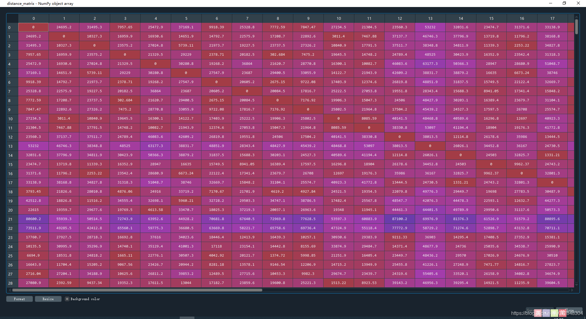
敲黑板,我定义的这个函数haversine就是用来求解任意两点之间距离的函数,下面这行代码很关键
distance_matrix = squareform(pdist(df, (lambda u, v: haversine(u, v))))
计算结果如下,矩阵的意义是任意两点之间的距离,对角线上全为0
再看聚类参数
db = DBSCAN(eps=500, min_samples=10, metric='precomputed').fit_predict(distance_matrix)
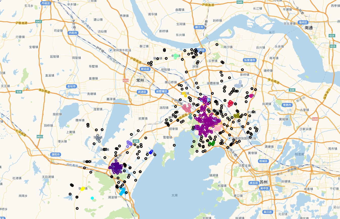
这里的metric='precomputed’不再是欧式距离,后面也不再是fit函数,而是fit_predict函数,用这种方法呢,就将原来的欧式距离换成了实际的距离,当然。看看聚类效果:
由于点太多,我把噪声点去掉了。
再看看用相同的数据点,我用原始的聚类算发的聚类效果:
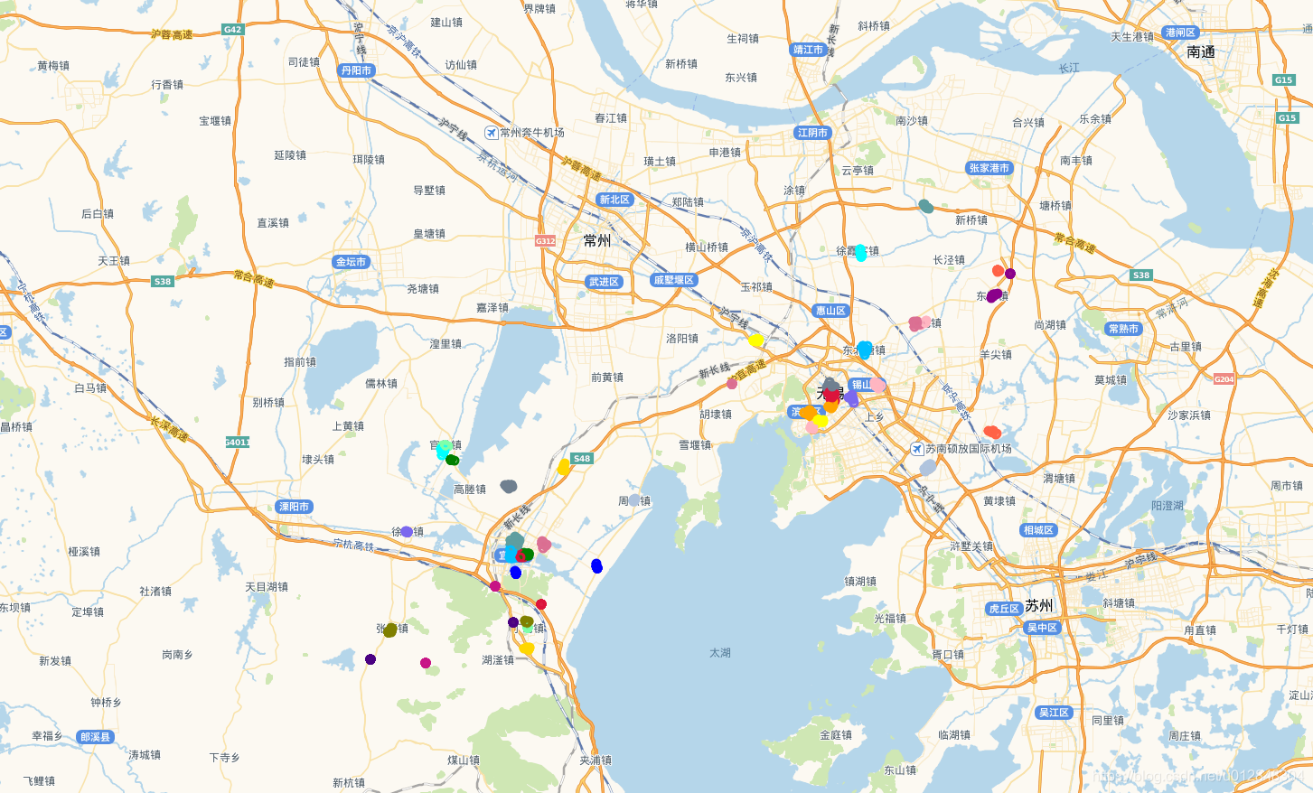
我感觉差不多。
写到这里,其实内容已经写完了。
但是还有一个问题并没有解决,就是DBSCAN聚类参数,到底该怎么输入,难道真要一个个去试吗,有没有好的办法来解决呢,能不能自适应呢,肯定是可以的。
继续看下面的内容。
轮廓系数调整输入参数
在前面的代码中,一直有一行代码我没解释
score = metrics.silhouette_score(data, labels)
就是这行代码,从变量的定义来看,我定义了一个得分,metrics.silhouette_score是机器学习中轮廓系数的计算函数,也就是说我可以用这个函数来计算模型的得分,是怎么一个计算过程呢,我这里详细介绍一下:
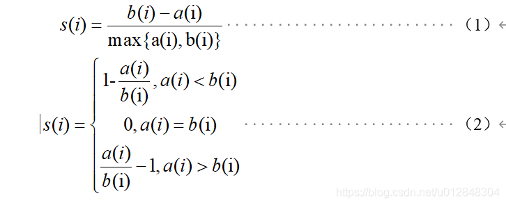
在聚类算法中,可以使用轮廓系数(Silhouette Coefficient)对聚类样本的聚类效果进行评估,轮廓系数的计算模型如式(1)、式(2)所示。
上式中, s(i)为样本i的轮廓系数,该值越接近1,说明样本i聚类越合理,越接近-1,说明样本i更应该分类到另外的簇,越接近0,说明样本i在两个簇的边界上; a(i)为样本i到簇内不相似度,为该样本同簇其他样本的平均距离,该值越小,说明该样本越应被聚类到该簇;b(i) 为样本i的簇间不相似度,计算公式如式(3)所示。
式(3)中, bij表示样本i到某簇Cj 所有样本的平均距离。
根据所有样本的轮廓系数计算平均值,即可得到当前聚类模型的总体轮廓系数值,并依据该值确定输入参数。

注:以上内容来源于本人论文。
就是说,我可以根据轮廓系数来不断调整我的输入参数,直到找到轮廓系数最大值对应的输入参数,这样就找到了最佳参数了。
上流程图
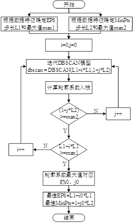
流程图解释的很清楚了,我再上一段代码来解释调参过程。
res = []
# 迭代不同的eps值
for eps in np.arange(0.001,0.13,0.001):
    # 迭代不同的min_samples值
    for min_samples in range(2,11):
        dbscan = DBSCAN(eps = eps, min_samples = min_samples)
        # 模型拟合
        dbscan.fit(data)
        # 统计各参数组合下的聚类个数(-1表示异常点)
        n_clusters = len([i for i in set(dbscan.labels_) if i != -1])
        # 异常点的个数
        outliners = np.sum(np.where(dbscan.labels_ == -1, 1,0))
        # 统计每个簇的样本个数
        # stats = pd.Series([i for i in dbscan.labels_ if i != -1]).value_counts()
        # 计算聚类得分
        try:
            score = metrics.silhouette_score(data, dbscan.labels_)
        except:
            score = -99
        res.append({'eps':eps,'min_samples':min_samples,'n_clusters':n_clusters,'outliners':outliners, 'score':score})
# 将迭代后的结果存储到数据框中
result = pd.DataFrame(res)
相关的参数解释如下:
- eps的调参范围是[0.001,0.13],这个参数是根据数据特征来获取的,就是说得对数据有一定的认识才能确定调参范围,循环的步长是0.001,意思就是说,最小距离半径是0.001,最大是0.13,注意,这里用的是欧式距离计算;
- min_samples的调参范围是[2,11],一个簇内至少得包含两个点吧,如果最少点超过了11,那么会将所有的点聚成同一个类,参数就是这么定的,循环步长是1。
这样就完成了整个调参过程。
实际效果如何和,我只能说不理想。
我们来看一下,上面我认为聚类较好的参数的轮廓系数:
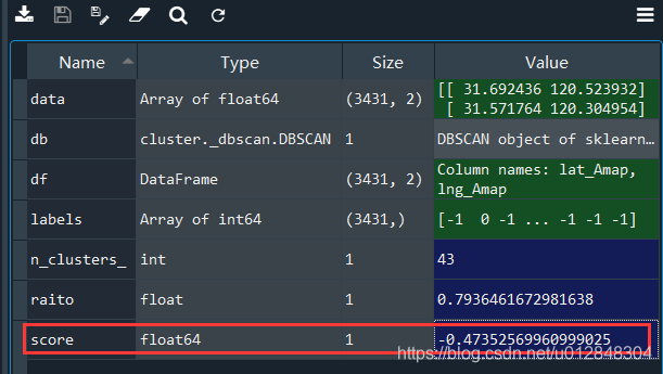
得分是个负数。。而很多接近于1的轮廓系数对应的聚类效果简直一塌糊涂,不过我尝试了一些其他的数据,总体来说,轮廓系数还是可以来评价的。
至此,相关技术细节都已介绍完毕。
不过大家要注意一下,folium包在目前的使用过程中,可能会出现一些问题,我出现的问题就是地图上的标注没法正常显示,可以用下面的方法来解决:
把folium.py里面原来的http://code.jquery.com/jquery-1.12.4.min.js,替换成https://cdn.bootcdn.net/ajax/libs/jquery/1.12.4/jquery.min.js
总结
列一下博客中的技术细节:
- DBSCAN聚类算法原理
- Python 机器学习实现DBSCAN聚类过程
- 应用欧式距离实现聚类
- 通过实际计算实际距离得到距离矩阵实现聚类
- 聚类结果上地图
- 根据轮廓系数调整聚类参数
这篇博客,总结了博主近半年内研究的东西,涉及到GIS、机器学习,内容比较多。
注:本文为原创文章,且部分内容涉及知识产权归属,仅供学习讨论,若要引用或转载,请注明本文出处


 1025
1025


 被折叠的 条评论
为什么被折叠?
被折叠的 条评论
为什么被折叠?
 到【灌水乐园】发言


