梯度下降求解逻辑回归2（代码编写以及三种梯度下降对比）

*上一篇是理论知识、背景介绍以及大体的实现方向，这一篇是具体代码实现

代码编写

我们的功能模块：

• 写出sigmoid函数，返回被录取的概率，即映射到概率

$$g(z) = \frac{1}{1+e^{-z}}$$

• 写出model函数，返回预测结果值，即X（样本值）与theta的矩阵相乘结果

$$\begin{array}{ccc} \begin{pmatrix}\theta_{0} & \theta_{1} & \theta_{2}\end{pmatrix} & \times & \begin{pmatrix}1\\ x_{1}\\ x_{2} \end{pmatrix}\end{array}=\theta_{0}+\theta_{1}x_{1}+\theta_{2}x_{2}$$

• 写出cost函数，实现计算损失函数，目的是度量预测值与真实值的拟合程度

将对数似然函数去负号

$$D(h_\theta(x), y) = -y\log(h_\theta(x)) - (1-y)\log(1-h_\theta(x))$$
求平均损失
$$J(\theta)=\frac{1}{n}\sum_{i=1}^{n} D(h_\theta(x_i), y_i)$$

• 写出gradient函数，来计算每个样本的梯度方向，即学习方向，梯度下降的方向
  

  $$\frac{\partial J}{\partial \theta_j}=-\frac{1}{m}\sum_{i=1}^n (y_i - h_\theta (x_i))x_{ij}$$

• 设置停止策略模式

• descent函数，实现参数 $\theta$ 的更新

• accuracy函数，计算精度

整体代码如下：

import os
import time
import numpy as np
import pandas as pd
import matplotlib.pyplot as plt
import numpy.random
%matplotlib inline

def sigmoid(z):
    return 1 / (1 + np.exp(-z))

def model(X, theta):
    # 预测函数  得到预测结果  矩阵相乘
    return sigmoid(np.dot(X, theta.T))

def cost(X, y, theta):
    # 计算损失函数 按照公式
    left = np.multiply(-y, np.log(model(X, theta)))  # 左边的连乘
    right = np.multiply((1 - y), np.log(1 - model(X, theta))) # 右边的连乘
    return np.sum(left - right) / (len(X))

def gradient(X, y, theta):
    # 求解梯度 grad为 theta梯度的更新值
    grad = np.zeros(theta.shape)
    error = (model(X, theta) - y).ravel()
    for j in range(len(theta.ravel())):

        temp = np.multiply(error, X[:,j])
        grad[0, j] = np.sum(temp) / len(X)

    return grad

# 设定三种停止策略 分别是按迭代次数、按损失函数的变化量、按梯度的变化量
STOP_ITER = 0
STOP_COST = 1
STOP_GRAD = 2

# threshold为指定阈值
def stopCriterion(stype, value, threshold):
    #设定三种不同的停止策略
    if stype == STOP_ITER:        
        return value > threshold # 按迭代次数停止

    elif stype == STOP_COST:
        return abs(value[-1]-value[-2]) < threshold  # 按损失函数是否改变停止

    elif stype == STOP_GRAD:
        return np.linalg.norm(value) < threshold # 按梯度大小停止



def shuffleData(data):
    # 洗牌 防止数据有一定的排列规律
    np.random.shuffle(data)
    cols = data.shape[1]
    X = data[:, 0:cols-1]
    y = data[:, cols-1:]
    return X, y

def descent(data, theta, batchSize, stopType, thresh, alpha):
    # 最主要的函数 梯度下降求解
    # batchSize：为1代表随机梯度下降  为整体值表示批量梯度下降  为某一数值时表示小批量梯度下降
    # stopType 停止策略类型
    # thresh 阈值
    # alpha 学习率

    init_time = time.time() 
    i = 0 # 迭代次数
    k = 0 # batch 迭代数据的初始量
    X, y = shuffleData(data)
    grad = np.zeros(theta.shape) # 计算的梯度
    costs = [cost(X, y, theta)] # 损失值

    while True:
        # batchSize为指定的梯度下降策略 
        grad = gradient(X[k:k+batchSize], y[k:k+batchSize], theta)
        k += batchSize #取batch数量个数据
        if k >= n: 
            k = 0 
            X, y = shuffleData(data) #重新洗牌
        theta = theta - alpha*grad # 参数更新
        costs.append(cost(X, y, theta)) # 计算新的损失
        i += 1 

        if stopType == STOP_ITER:       
            value = i

        elif stopType == STOP_COST:     
            value = costs

        elif stopType == STOP_GRAD:     
            value = grad

        if stopCriterion(stopType, value, thresh): 
            break

    return theta, i-1, costs, grad, time.time() - init_time

def runExpe(data, theta, batchSize, stopType, thresh, alpha):
    # 损失率与迭代次数的展示函数
    theta, iter, costs, grad, dur = descent(data, theta, batchSize, stopType, thresh, alpha)
    name = "Original" if (data[:,1]>2).sum() > 1 else "Scaled"
    name += " data - learning rate: {} - ".format(alpha)

    if batchSize == n: 
        strDescType = "Gradient"

    elif batchSize == 1:  
        strDescType = "Stochastic"

    else: 
        strDescType = "Mini-batch ({})".format(batchSize)

    name += strDescType + " descent - Stop: "

    if stopType == STOP_ITER: 
        strStop = "{} iterations".format(thresh)

    elif stopType == STOP_COST: 
        strStop = "costs change < {}".format(thresh)

    else: 
        strStop = "gradient norm < {}".format(thresh)

    name += strStop
    print("***{}\nTheta: {} - Iter: {} - Last cost: {:03.2f} - Duration: {:03.2f}s".format(
        name, theta, iter, costs[-1], dur))
    fig, ax = plt.subplots(figsize=(12,4))
    ax.plot(np.arange(len(costs)), costs, 'r')
    ax.set_xlabel('Iterations')
    ax.set_ylabel('Cost')
    ax.set_title(name.upper() + ' - Error vs. Iteration')

    return theta

path = 'data' + os.sep + 'LogiReg_data.txt'
# 载入数据（训练集）
pdData = pd.read_csv(path, header=None, names=['Exam1', 'Exam2', 'Admitted'])

pdData.insert(0, 'Ones', 1) # in a try / except structure so as not to return an error if the block si executed several times
orig_data = pdData.as_matrix() 
cols = orig_data.shape[1]
X = orig_data[:,0:cols-1]
y = orig_data[:,cols-1:cols]

theta = np.zeros([1, 3])

成果展示

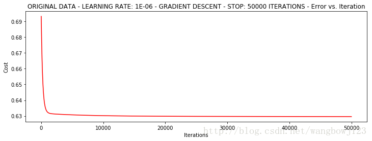
首先我们执行批量梯度下降策略，并设置迭代次数为停止策略：

# 设定迭代次数为50000次
n = 100
runExpe(orig_data, theta, n, STOP_ITER, thresh=50000, alpha=0.000001)

结果如下：

***Original data - learning rate: 1e-06 - Gradient descent - Stop: 50000 iterations
Theta: [[-0.00341509 0.01035718 0.00056757]] - Iter: 50000 - Last cost: 0.63 - Duration: 9.24s
array([[-0.00341509, 0.01035718, 0.00056757]])

之后再设置为随机梯度下降策略，并设置迭代次数为停止策略：

# 为了快速 设置迭代次数为 5000
runExpe(orig_data, theta, 1, STOP_ITER, thresh=5000, alpha=0.001)

结果如下：

***Original data - learning rate: 0.001 - Stochastic descent - Stop: 5000 iterations
Theta: [[-0.38444806 -0.00892323 -0.02050201]] - Iter: 5000 - Last cost: 1.64 - Duration: 0.33s
array([[-0.38444806, -0.00892323, -0.02050201]])

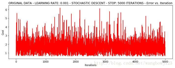
可以看出我们的损失函数非常不稳定，那么我们把学习率调低一些再看看结果：

runExpe(orig_data, theta, 1, STOP_ITER, thresh=15000, alpha=0.000002)

***Original data - learning rate: 2e-06 - Stochastic descent - Stop: 15000 iterations
Theta: [[-0.00202099 0.01001901 0.000949 ]] - Iter: 15000 - Last cost: 0.63 - Duration: 0.91s
array([[-0.00202099, 0.01001901, 0.000949 ]])

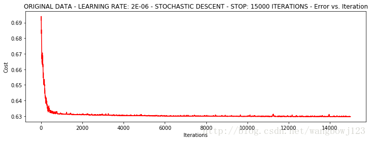
可以看出来损失函数基本收敛，速度是挺快的，但是整体不是很稳定。
我们再试试小批量梯度下降策略：

# 设置迭代次数为 15000次结束
runExpe(orig_data, theta, 16, STOP_ITER, thresh=15000, alpha=0.001)

结果如下：

***Original data - learning rate: 0.001 - Mini-batch (16) descent - Stop: 15000 iterations
Theta: [[-1.03877323 0.02183561 0.01401876]] - Iter: 15000 - Last cost: 0.60 - Duration: 1.17s
array([[-1.03877323, 0.02183561, 0.01401876]])

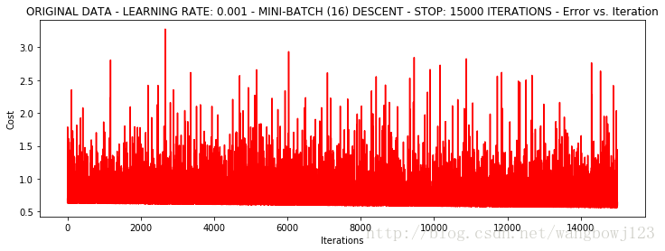
结果很是糟糕，浮动仍然比较大，我们来尝试下对数据进行标准化 将数据按其属性(按列进行)减去其均值，然后除以其方差。最后得到的结果是，对每个属性/每列来说所有数据都聚集在0附近，方差值为1（数据标准化）。
至于为什么要进行数据标准化，我会再以后的文章里进行讨论。

from sklearn import preprocessing as pp
# 引入sklearn 进行数据处理
scaled_data = orig_data.copy()
scaled_data[:, 1:3] = pp.scale(orig_data[:, 1:3])

之后，我们再进行批量梯度下降策略的执行：

# 设置迭代5000次
runExpe(scaled_data, theta, n, STOP_ITER, thresh=5000, alpha=0.001)

结果如下：

***Scaled data - learning rate: 0.001 - Gradient descent - Stop: 5000 iterations
Theta: [[ 0.3080807 0.86494967 0.77367651]] - Iter: 5000 - Last cost: 0.38 - Duration: 1.03s
array([[ 0.3080807 , 0.86494967, 0.77367651]])

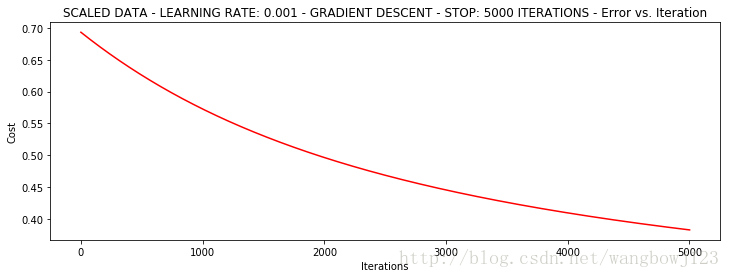
它好多了！原始数据，只能达到达到0.61，而我们得到了0.38个在这里！ 所以对数据做预处理是非常重要的
但是我们对最终结果不是很满意，迭代次数似乎有些少了。这时，我们再改变停止策略试一下：

# 使用批量梯度下降策略并设置以梯度变化量为停止策略
runExpe(scaled_data, theta, n, STOP_GRAD, thresh=0.02, alpha=0.001)

结果如下：

***Scaled data - learning rate: 0.001 - Gradient descent - Stop: gradient norm < 0.02
Theta: [[ 1.0707921 2.63030842 2.41079787]] - Iter: 59422 - Last cost: 0.22 - Duration: 12.02s
array([[ 1.0707921 , 2.63030842, 2.41079787]])

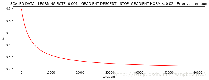
可以看出来更多的迭代使得损失下降的更多！，我们最终的损失达到了0.22！

再试试随机梯度下降策略：

# 设置为随机梯度下降并使得停止策略为梯度的变化
theta = runExpe(scaled_data, theta, 1, STOP_GRAD, thresh=0.002/5, alpha=0.001)

结果如图：

***Scaled data - learning rate: 0.001 - Stochastic descent - Stop: gradient norm < 0.0004
Theta: [[ 1.1491578 2.7927126 2.56466683]] - Iter: 72562 - Last cost: 0.22 - Duration: 5.36s

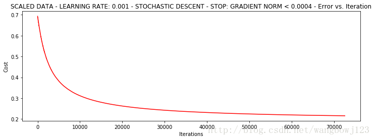
最终损失也是0.22，同时耗费时间也比批量梯度下降少了一半还多！但是迭代次数却增加了。
可以发现使用随机梯度下降使得下降更快了，但是迭代次数却增加了，所以我们使用小批量梯度下降：

# 使用小批量梯度下降（每次取16个数据） 并设置梯度改变的阈值为 0.002*2
theta = runExpe(scaled_data, theta, 16, STOP_GRAD, thresh=0.002*2, alpha=0.001)

***Scaled data - learning rate: 0.001 - Mini-batch (16) descent - Stop: gradient norm < 0.004
Theta: [[ 1.15563838 2.8082394 2.57601557]] - Iter: 1252 - Last cost: 0.22 - Duration: 0.14s

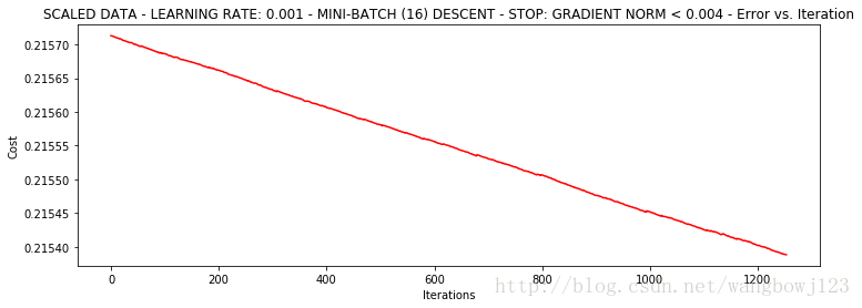
可以很神奇的发现：我们的曲线并不光滑，却最终收敛在了0.22，并且迭代次数、运行时间都优于上面两种策略！
因此我们可以得出结论：在本案例中使用小批量梯度下降策略时相对较优的。

精确度的测量

最后我们再用小批量梯度下降所预测的数据来和真实数据做对比，测量一下精度：

#设定阈值
def predict(X, theta):
    return [1 if x >= 0.5 else 0 for x in model(X, theta)]

scaled_X = scaled_data[:, :3]
y = scaled_data[:, 3]
predictions = predict(scaled_X, theta)
correct = [1 if ((a == 1 and b == 1) or (a == 0 and b == 0)) else 0 for (a, b) in zip(predictions, y)]
accuracy = (sum(map(int, correct)) % len(correct))
print ('accuracy = {0}%'.format(accuracy))

结果为：

accuracy = 89%

结语

本博客是对唐宇迪教学视频的大体总结，包含了本人对算法的理解。
学完这个小案例之后，对梯度下降求解逻辑回归有了一个大体而感性的认识，希望能作为入门的一个小小教程。