


In this article, we will build a logistic regression model for classifying whether a patient has diabetes or not. The main focus here is that we will only use python to build functions for reading the file, normalizing data, optimizing parameters, and more. So you will be getting in-depth knowledge of how everything from reading the file to make predictions works.
在本文中,我们将建立一个Logistic 回归模型来对患者是否患有糖尿病进行分类。 这里的主要重点是,我们将仅使用python构建用于读取文件,规范化数据,优化参数等的函数。 因此,您将深入了解从读取文件到进行预测的所有工作方式。
If you are new to machine learning, or not familiar with logistic regression or gradient descent, don’t worry I’ll try my best to explain these in layman’s terms. There are more tutorials out there that explain the same concepts. But what makes this tutorial unique is its short and beginners friendly high-level description of the code snippets. So, let's start by looking at some theoretical concepts that are important in order to understand the working of our model.
如果您是机器学习的新手,或者对逻辑回归或梯度 下降不熟悉,请不要担心,我会尽力用外行的术语解释这些问题。 有更多的教程可以解释相同的概念。 但是,使本教程与众不同的是它对代码片段的简短且对初学者友好的高级描述。 因此,让我们从一些重要的理论概念入手,以理解我们模型的工作原理。
逻辑回归 (Logistic Regression)
Logistic Regression is the entry-level supervised machine learning algorithm used for classification purposes. It is one of those algorithms that everyone should be aware of. Logistic Regression is somehow similar to linear regression but it has different cost function and prediction function(hypothesis).
Logistic回归是用于分类目的的入门级有监督机器学习算法。 这是每个人都应该意识到的算法之一。 Logistic回归在某种程度上类似于线性回归,但具有不同的成本 函数和预测 函数 (假设)。

乙状结肠功能 (Sigmoid function)
It is the activation function that squeezes the output of the function in the range between 0 and 1 where values less than 0.5 represent class 0 and values greater than or equal to 0.5 represents class 1.
激活函数将函数的输出压缩在0和1之间的范围内,其中小于0.5的值表示0类,而大于或等于0.5的值表示1类。

成本函数 (Cost Function)
Cost function finds the error between the actual value and predicted value of our algorithm. It should be as minimum as possible. In the case of linear regression, the formula is:-
成本函数可以找到我们算法的实际值和预测值之间的误差。 它应该尽可能的小。 在线性回归的情况下,公式为:
But this formula cannot be used for logistic regression because the hypothesis here is a nonconvex function that means there are chances of finding the local minima and thus avoiding the global minima. If we use the same formula then our plot will look like this:-
但是此公式不能用于逻辑 回归,因为此处的假设是一个非凸函数,这意味着有机会找到局部最小值,从而避免了全局最小值。 如果我们使用相同的公式,则图将如下所示:-

So, in order to avoid this, we have smoothened the curve with the help of log and our cost function will look like this:-
因此,为了避免这种情况,我们在对数的帮助下对曲线进行了平滑处理 ,成本函数如下所示:

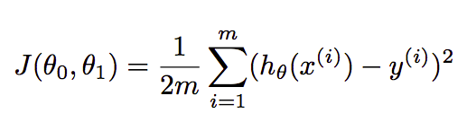
where m=number of examples or rows in the dataset, xᶦ=feature values of iᵗʰ example, yᶦ=actual outcome of iᵗʰ example. After using this, our plot for the cost function will look like this:-
其中,m =数据集中示例或行的数量,x = i实例的特征值,y = i实例的实际结果。 使用此函数后,成本函数的图将如下所示:-

梯度下降 (Gradient Descent)
Our aim in any ML algorithm is to find the set of parameters that minimizes the cost function. And for automatically finding the best set of parameters we use optimization techniques. One of them is gradient descent. In this, we start with random values of parameters(in most cases zero) and then keep changing the parameters to reduce J(θ₀,θ₁) or cost function until we end up at a minimum. The formula for the same is:-
在任何ML算法中,我们的目标都是找到使 成本 函数 最小化的参数集。 为了自动找到最佳的参数集,我们使用了优化技术。 其中之一是梯度下降。 在此,我们用的参数随机值开始(在大多数情况下为零 ),然后保持改变参数以减少Ĵ(θ₀,θ₁)或成本函数,直到我们在最小结束。 相同的公式是:

It looks exactly the same as that of linear regression but the difference is of the hypothesis(hθ(x)) as it uses sigmoid function as well.
它看起来与线性回归完全相同,但是差异在于假设( hθ(x) ),因为它也使用了S型函数。
That’s a lot of theory, I know but that was required to understand the following code snippets. And I have only scratched the surface, so please google the above topics for in-depth knowledge.
我知道,这是很多理论,但这是理解以下代码段所必需的。 而且我只是从头开始,因此请在Google上面的主题中进行深入了解。
先决条件: (Prerequisites:)
I assume that you are familiar with python and already have installed the python 3 in your systems. I have used a jupyter notebook for this tutorial. You can use the IDE of your like. All required libraries come inbuilt in anaconda suite.
我假设您熟悉python,并且已经在系统中安装了python 3 。 我在本教程中使用了jupyter笔记本 。 您可以使用自己喜欢的IDE 。 所有必需的库都内置在anaconda套件中。
让我们编码 (Let’s Code)
Okay, so I have imported CSV, numpy(for majorly dot product only), and math for performing log and exponential calculations.
好的,我已经导入了CSV,numpy(仅用于点产品)和用于执行对数和指数计算的数学运算。
读取文件 (Read the File)
Firstly, we have defined the function read_filefor reading the dataset itself. Here, the file is opened with with so we don't have to close it and stored it in the reader variable. Then we loop over reader and append each line in the list named dataset. But the loaded data is of string format as shown in screenshot below.
首先,我们定义了函数read_file来读取数据集本身。 在这里,文件打开与with ,所以我们不必将其关闭并将其存储在阅读器的变量。 然后,我们遍历reader ,并将每行追加到名为dataset的列表中。 但是加载的数据为字符串格式,如下面的屏幕快照所示。

将String转换为Float (Convert String to Float)
The string_to_float function here helps to convert all string values to float in order to perform calculations on it. We simply loop on each row and column and convert every entry from string to float.
这里的string_to_float函数有助于将所有字符串值转换为float以便对其执行计算。 我们只需循环遍历每一行和每一列,然后将每个条目从字符串转换为浮点数即可。

查找最小最大 (Find Min Max)
Now, in order to perform normalization or getting all values on the same scale, we have to find the minimum and maximum values from each column. Here in function, we have loop column-wise and append the max and min of every column in minmax list. Obtained values are shown in the screenshot below.
现在,为了执行归一化或以相同比例获得所有值,我们必须从每一列中找到最小值和最大值 。 在函数中,我们按列循环,并在minmax列表中追加每列的max和min。 获得的值显示在下面的屏幕快照中。

正常化 (Normalization)
Now, we have looped over every value in the dataset and subtract minimum value (of that column) from it and divide it with the difference of max and min of that column. The screenshot below represents the normalized values of a single row example.
现在,我们遍历了数据集中的每个值,并从中减去(该列的)最小值,然后除以该列的最大值和最小值之差。 下面的屏幕快照表示单行示例的规范化值。

Train Test Split
火车测试拆分
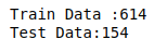
Here, train_test function helps to create training and testing datasets. We have used shuffle from random module to shuffle the whole dataset. Then we slice the dataset to 80% and store it in train_data and the remaining 20% in test_data . The size of both sets is shown below.
在这里, train_test函数有助于创建训练和测试数据集。 我们使用shuffle从随机模块洗牌整个数据集。 然后我们将数据集切成80%并将其存储在train_data ,其余20%存储在test_data 。 两组的尺寸如下所示。
准确性 (Accuracy)
This accuracy_check function will be used to check the accuracy of our model. Here, we simply looped over the length of the actual or predicted list as both are of the same length and if the value at the current index of both are same, we increase the count c . Then just divide that count c with the length of the actual or predicted list and multiply by 100 to get the accuracy %.
此accuracy_check函数将用于检查模型的准确性。 在这里,我们简单地遍历了实际列表或预测列表的长度,因为两者的长度相同,并且如果两者当前索引处的值相同,我们将增加计数c 。 然后,只需将计数c除以实际或预测列表的长度,然后乘以100即可得出精度%。
预测或假设功能 (Prediction or Hypothesis Function)
Yes, here we have imported numpy to calculate dot product but function for that can also be made. math for calculating exponential. The prediction function is our hypothesis function that takes the whole row and parameters as arguments. We have then initialized hypothesis variable with θo and we looped over every row element ignoring the last as it is the target y variable and added xᵢ*θ(i+1) (i+1 is in subscript) to hypothesis variable. After that, comes the sigmoid function 1/(1+exp(-hypothesis)) that squeezes the value in the range of 0–1.
是的,这里我们导入了numpy来计算点积,但是也可以实现该功能。 用于计算指数的math 。 prediction函数是我们的假设函数,它将整个行和参数作为参数。 然后,我们用θo初始化了假设变量,并循环了每个行元素,而忽略了最后一个,因为它是目标y变量,并向y变量中添加了xᵢ*θ(i + 1)(i + 1在下标中)。 之后,出现了sigmoid函数1 /(1 + exp(-hypothesis)),它将值压缩在0–1的范围内。
成本函数 (Cost Function)
We don’t necessarily need this function to get our model worked but it is good to calculate the cost with every iteration and plot that. Incost_function we have looped over every row in the dataset and calculated costof that row with the formula described above then add it to the cost variable. Finally, the average cost is returned.
我们不一定需要此函数才能使模型工作,但是在每次迭代中计算成本并将其绘制出来是很好的。 在cost_function我们遍历了数据集中的每一行,并使用上述公式计算了该行的cost ,然后将其添加到cost变量中。 最后,返回平均成本。
优化技术 (Optimization Technique)
Here, we have used gradient_descent for automatically finding the best set of parameters for our model. This function takes dataset, epochs(number of iterations), and alpha(learning rate) as arguments. In the function, cost_history is initialized to append the cost after every epoch and parametersto hold the set of parameters(no. of paramters=features+1). After that, we started a loop to repeat the process of finding the parameters. The inner loop is used to iterate over every row in the dataset. Here gradient term is different for θo due to partial derivative of the cost function, that's why it is calculated separately and added to 0th position in parameters list, then other parameters are calculated using other feature values of row(ignoring last target value) and added to their respective position in the parameters list. The same process repeats for every row. After that 1 epoch is completed and cost_function is called with the calculated set of parameters and the value obtained is appended to cost_history .
在这里,我们使用了gradient_descent为我们的模型自动找到最佳的参数集。 此函数将数据集 , 时期 (迭代数)和alpha (学习率)作为参数。 在该函数中,初始化cost_history以在每个时期和parameters之后追加成本,以保存参数集(paramters的数量=功能+1)。 之后,我们开始循环以重复查找参数的过程。 内部循环用于迭代数据集中的每一行。 由于成本函数的偏导数,因此θo的梯度项有所不同,这就是为什么将其单独计算并添加到参数列表中的第0个位置,然后使用row的其他特征值计算其他参数(忽略最后一个目标值)并将其相加的原因到它们在参数列表中各自的位置。 每行重复相同的过程。 在那之后的1个时期完成,使用计算出的参数集调用cost_function ,并将获得的值附加到cost_history 。
组合算法 (Combining Algorithm)
Here, we have imported matplotlib.pyplot just to draw the cost plot. So it is not necessary. In algorithm function, we are calling the gradient_descent with epochs=1000 and learning_rate = 0.001. After that, making predictions on our testing dataset. round is used to round off the obtained predicted values(i.e. 0.7=1,0.3=0). Then, accuracy_check is called to get the accuracy of the model. At last, we have plotted the iterations v/s cost plot.
在这里,我们导入了matplotlib.pyplot只是为了绘制成本图。 因此没有必要。 在algorithm函数中,我们以epochs = 1000和learning_rate = 0.001的方式调用gradient_descent 。 之后,对我们的测试数据集进行预测。 round用于舍入所获得的预测值(即0.7 = 1,0.3 = 0)。 然后, accuracy_check被调用,以获得该模型的准确性。 最后,我们绘制了迭代数与成本的关系图。
放在一起 (Putting Everything Together)
Just to have a proper structure, we have put all the functions in a single combine function. We were able to achieve an accuracy of around 78.5% which can be further improved by hyper tuning the model. The plot below also proves that our model is working correctly as cost is decreasing with an increase in the number of iterations.
为了具有适当的结构,我们将所有功能都放在一个combine功能中。 我们能够达到大约78.5%的准确度,可以通过对模型进行超调来进一步提高其准确性。 下图还证明了,随着迭代次数增加,成本降低,我们的模型可以正常工作。

结论 (Conclusion)
We have successfully build a Logistic Regression model from scratch without using pandas, scikit learn libraries. We have achieved an accuracy of around 78.5% which can be further improved. Also, we can leave numpy and built a function for calculating dot products. Although we will use sklearn, it good to know the inner working as well. 😉
我们已经从零开始成功构建了Logistic 回归模型,而无需使用pandas , scikit 学习库。 我们已经达到了约78.5%的准确度,可以进一步提高。 另外,我们可以离开numpy并构建一个用于计算点积的函数。 尽管我们将使用sklearn,但最好也了解内部工作原理。 😉
The source code is available on GitHub. Please feel free to make improvements.
Thank you for your precious time.😊And I hope you like this tutorial.
谢谢您的宝贵时间。😊我希望您喜欢本教程。
Also, check my tutorial on a Gradient Descent v/s Normal Equation
另外,请查看我的有关梯度下降v / s正态方程的教程


 454
454

 被折叠的 条评论
为什么被折叠?
被折叠的 条评论
为什么被折叠?
 到【灌水乐园】发言


