创建dqn的深度神经网络_深度Q网络（DQN）-I

创建dqn的深度神经网络

深层加固学习介绍— 15 (DEEP REINFORCEMENT LEARNING EXPLAINED — 15)

In the previous post, we have presented solution methods that represent the action-values in a small table. We referred to this table as a Q-table. In the next three posts of the “Deep Reinforcement Learning Explained” series, we will introduce the reader to the idea of using neural networks to expand the size of the problems that we can solve with reinforcement learning presenting the Deep Q-Network (DQN), that represents the optimal action-value function as a neural network, instead of a table. In this post, we will do an overview of DQN as well as introduce the OpenAI Gym framework of Pong. In the next two posts, we will present the algorithm and its implementation.

在上一篇文章中 ，我们介绍了在一个小表中表示操作值的解决方法。 我们将此表称为Q表 。 在“ 深度强化学习的说明 ”系列的后三篇文章中，我们将向读者介绍使用神经网络来扩展我们可以通过提出深度Q网络(DQN)的强化学习解决的问题的规模的想法。 ，代表最佳行动价值函数作为神经网络(而不是表格)。 在本文中，我们将概述DQN并介绍Pong的OpenAI Gym框架 。 在接下来的两篇文章中，我们将介绍该算法及其实现。

Atari 2600游戏 (Atari 2600 games)

The Q-learning method that we have just covered in previous posts solves the issue by iterating over the full set of states. However often we realize that we have too many states to track. An example is Atari games, that can have a large variety of different screens, and in this case, the problem cannot be solved with a Q-table.

我们在之前的文章中已经介绍了Q学习方法，它通过遍历整个状态来解决此问题。 但是，我们常常意识到我们有太多的州要追踪。 Atari游戏就是一个例子，它可以具有多种不同的屏幕，在这种情况下，用Q表无法解决问题。

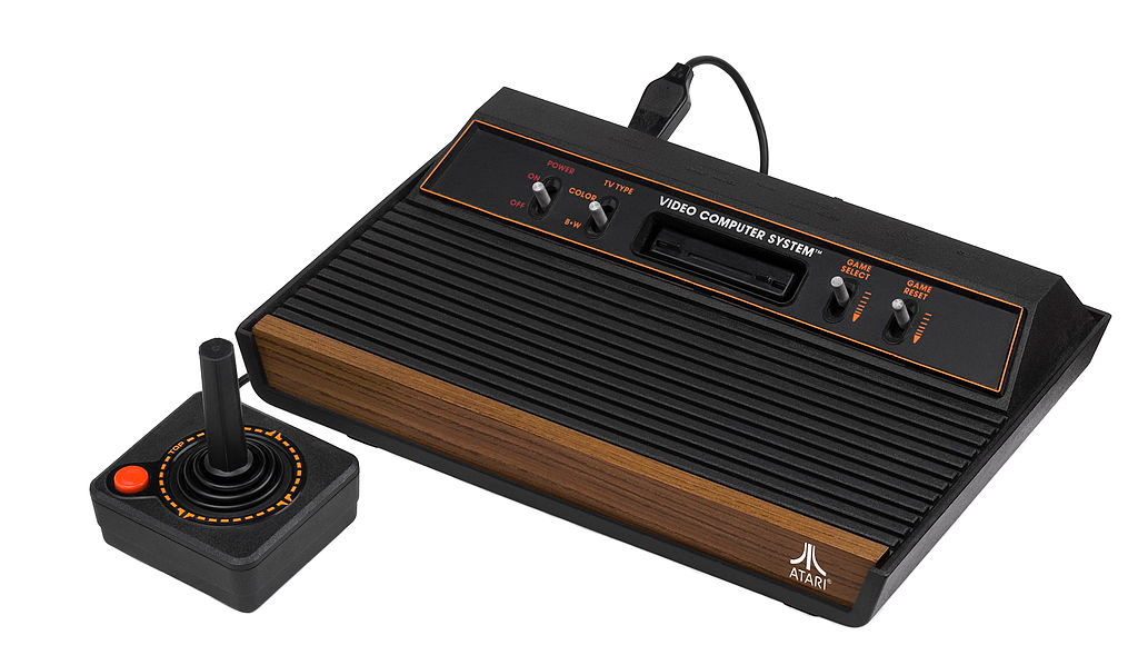
The Atari 2600 game console was very popular in the 1980s, and many arcade-style games were available for it. The Atari console is archaic by today’s gaming standards, but its games still are challenging for computers and is a very popular benchmark within RL research (using an emulator)

Atari 2600游戏机在1980年代非常流行，并且有许多街机风格的游戏可供使用。 Atari控制台按当今的游戏标准来说是过时的，但是其游戏仍然对计算机构成挑战，并且是RL研究(使用仿真器)中非常受欢迎的基准

Wikipedia) 维基百科 )

In 2015 DeepMind leveraged the so-called Deep Q-Network (DQN) or Deep Q-Learning algorithm that learned to play many Atari video games better than humans. The research paper that introduces it, applied to 49 different games, was published in Nature (Human-Level Control Through Deep Reinforcement Learning, doi:10.1038/nature14236, Mnih, and others) and can be found here.

2015年，DeepMind利用了所谓的Deep Q-Network(DQN)或Deep Q-Learning算法，该算法学会了比人类更好玩Atari视频游戏。 引入该方法的研究论文已应用于《自然》(《通过深度强化学习进行人的水平控制》，doi：10.1038 / nature14236，Mnih等人)上，并已在此处找到 ，该论文适用于49种不同的游戏。

The Atari 2600 game environment can be reproduced through the Arcade Learning Environment in the OpenAI Gym framework. The framework has multiple versions of each game but for the purpose of this post, the Pong-v0 Environment will be used.

可以通过OpenAI Gym框架中的Arcade学习环境来复制Atari 2600游戏环境。 该框架具有每个游戏的多个版本，但出于本文的目的，将使用Pong-v0环境。

We will study this algorithm because it really allows us to learn tips and tricks that will be very useful in future posts in this series. DeepMind’s Nature paper contained a table with all the details about hyperparameters used to train its model on all 49 Atari games used for evaluation. However, our goal here is much more modest: we want to solve just the Pong game.

我们将研究此算法，因为它确实允许我们学习在本系列的后续文章中将非常有用的提示和技巧。 DeepMind的Nature论文包含一张表格，其中包含用于在49个用于评估的Atari游戏中训练其模型的超参数的所有详细信息。 但是，我们这里的目标要适度得多：我们只想解决Pong游戏。

As we have done in some previous posts, the code presented in this post has been inspired by the code of Maxim Lapan who has written an excellent practical book on the subject.

就像我们在以前的文章中所做的一样，本文中的代码受到Maxim Lapan的代码的启发，Maxim Lapan编写了关于该主题的出色实用书籍 。

The entire code of this post can be found on GitHub and can be run as a Colab google notebook using this link.

这篇文章的完整代码可以在GitHub上找到 ， 也可以使用此链接作为Colab谷歌笔记本运行 。

Our previous examples for FrozenLake, or CartPole, were not demanding from a computation requirements perspective, as observations were small. However, from now on, that’s not the case. The version of code shared in this post converges to a mean score of 19.0 in 2 hours (using a NVIDIA K80). So don’t get nervous during the execution of the training loop. ;-)

从观察到的数据量很小，从计算需求的角度来看，我们以前针对FrozenLake或CartPole的示例并没有要求。 但是，从现在开始，情况并非如此。 这篇文章中共享的代码版本在2小时内平均得分达到19.0(使用NVIDIA K80)。 因此，在执行训练循环时不要紧张。 ;-)

傍 (Pong)

Pong is a table tennis-themed arcade video game featuring simple two-dimensional graphics, manufactured by Atari and originally released in 1972. In Pong, one player scores if the ball passes by the other player. An episode is over when one of the players reaches 21 points. In the OpenAI Gym framework version of Pong, the Agent is displayed on the right and the enemy on the left:

Pong是一款以乒乓球为主题的街机视频游戏，具有简单的二维图形，由Atari制造，最初于1972年发布。在Pong中，如果一名球传给另一名球员，则一名球员得分。 一个球员达到21分时，情节结束了。 在Pong的OpenAI Gym框架版本中 ，代理显示在右侧，而敌人显示在左侧：

torres.ai) torres.ai )

There are three actions an Agent (player) can take within the Pong Environment: remaining stationary, vertical translation up, and vertical translation down. However, if we use the method action_space.n we can realize that the Environment has 6 actions:

在乒乓环境中，特工(玩家)可以采取三种动作：保持静止，垂直平移和垂直平移。 但是，如果我们使用action_space.n方法，我们可以意识到环境有6个动作：

import gym
import gym.spacesDEFAULT_ENV_NAME = “PongNoFrameskip-v4”
test_env = gym.make(DEFAULT_ENV_NAME)print(test_env.action_space.n)6

Even though OpenAI Gym Pong Environment has six actions:

即使OpenAI Gym Pong Environment有六个动作：

print(test_env.unwrapped.get_action_meanings())[‘NOOP’, ‘FIRE’, ‘RIGHT’, ‘LEFT’, ‘RIGHTFIRE’, ‘LEFTFIRE’]

three of the six being redundant (FIRE is equal to NOOP, LEFT is equal to LEFTFIRE and RIGHT is equal to RIGHTFIRE).

六个中的三个是冗余的(FIRE等于NOOP，LEFT等于LEFTFIRE，RIGHT等于RIGHTFIRE)。

DQN概述 (DQN Overview)

At the heart of the Agent of this new approach, we found a deep neural network instead of a Q-table as we saw in the previous post. It should be noted that the Agent was only given raw pixel data, what a human player would see on screen, without access to the underlying game state, position of the ball, paddles, etc.

在这种新方法的Agent的核心，我们找到了一个深层的神经网络，而不是前面的文章中看到的Q表。 应该注意的是，Agent仅获得了原始像素数据，这是人类玩家在屏幕上看到的数据，而无法访问基础游戏状态，球的位置，球拍等。

As a reinforcement signal, it is fed back the change in game score at each time step. At the beginning, when the neural network is initialized with random values, it’s really bad, but overtime it begins to associate situations and sequences in the game with appropriate actions and learns to actually play the game well (that, without a doubt, the reader will be able to verify for himself with the code that will be presented in this series).

作为强化信号，它在每个时间步长反馈游戏分数的变化。 起初，当用随机值初始化神经网络时，这确实很糟糕，但是随着时间的推移，它开始将游戏中的情况和序列与适当的动作相关联，并学会实际玩游戏(毫无疑问，读者就能使用本系列中将介绍的代码进行自我验证)。

输入空间 (Input space)

Atari games are displayed at a resolution of 210 by 60 pixels, with 128 possible colors for each pixel:

Atari游戏以210 x 60像素的分辨率显示，每个像素有128种可能的颜色：

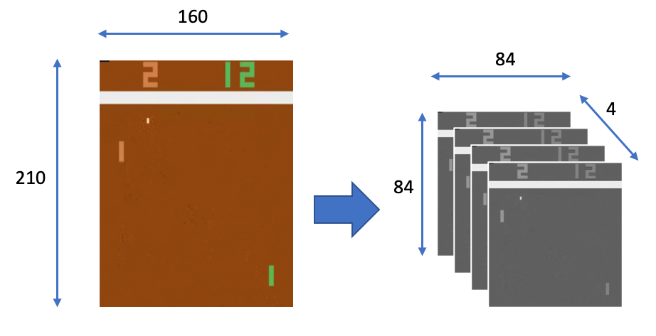
print(test_env.observation_space.shape)(210, 160, 3)

This is still technically a discrete state space but very large to process as it is and we can optimize it. To reduce this complexity, it is performed some minimal processing: convert the frames to grayscale, and scale them down to a square 84 by 84 pixel block. Now let’s think carefully if with this fixed image we can determine the dynamics of the game. There is certainly ambiguity in the observation, right? For example, we cannot know in which direction the ball is going). This obviously violates the Markov property.

从技术上讲，这仍然是一个离散的状态空间，但按原样处理却非常大，我们可以对其进行优化。 为了降低这种复杂性，它执行了一些最少的处理：将帧转换为灰度，然后将其按比例缩小为84 x 84像素块。 现在，让我们仔细考虑一下，是否可以使用此固定图像确定游戏的动力。 观察中肯定有歧义，对吗？ 例如，我们不知道球朝哪个方向前进。 这显然违反了马尔可夫财产 。

The solution is maintaining several observations from the past and using them as a state. In the case of Atari games, the authors of the paper suggested to stack 4 subsequent frames together and use them as the observation at every state. For this reason, the preprocessing stacks four frames together resulting in a final state space size of 84 by 84 by 4:

解决方案是保留过去的一些观察结果并将其用作状态。 对于Atari游戏，论文的作者建议将4个后续帧堆叠在一起，并在每个州将其用作观察值。 因此，预处理将四个帧堆叠在一起，最终状态空间大小为84 x 84 x 4：

torres.ai) torres.ai )

输出量 (Output)

Unlike until now we presented a traditional reinforcement learning setup where only one Q-value is produced at a time, the Deep Q-network is designed to produce in a single forward pass a Q-value for every possible action available in the Environment:

不同于现在为止，我们提出了一种传统的强化学习设置，即一次只产生一个Q值，而深度Q网络被设计为通过一次正向传递为环境中可用的每种可能动作产生一个Q值：

torres.ai) torres.ai )

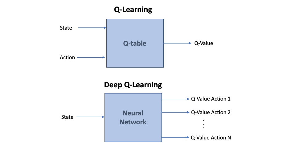
This approach of having all Q-values calculated with one pass through the network avoids having to run the network individually for every action and helps to increase speed significantly. Now, we can simply use this vector to take an action by choosing the one with the maximum value.

通过一次通过网络计算所有Q值的方法避免了必须为每个操作单独运行网络，并有助于显着提高速度。 现在，我们可以简单地使用此向量通过选择最大值来执行一项操作。

神经网络架构 (Neural Network Architecture)

The original DQN Agent used the same neural network architecture, for the all 49 games, that takes as an input an 84x84x4 image.

最初的DQN代理在所有49款游戏中都使用了相同的神经网络架构，将84x84x4的图像作为输入。

The screen images are first processed by three convolutional layers. This allows the system to exploit spatial relationships, and can sploit spatial rule space. Also, since four frames are stacked and provided as input, these convolutional layers also extract some temporal properties across those frames. Using PyTorch, we can code the convolutional part of the model as:

屏幕图像首先由三个卷积层处理。 这允许系统利用空间关系，并且可以划分空间规则空间。 而且，由于四个帧被堆叠并作为输入提供，因此这些卷积层还提取了那些帧上的某些时间属性。 使用PyTorch，我们可以将模型的卷积部分编码为：

nn.Conv2d(input_shape, 32, kernel_size=8, stride=4),
        nn.ReLU(),
        nn.Conv2d(32, 64, kernel_size=4, stride=2),
        nn.ReLU(),
        nn.Conv2d(64, 64, kernel_size=3, stride=1),
        nn.ReLU()

where input_shape is the observation_space.shape of the Environment.

其中input_shape是环境的observation_space.shape 。

The convolutional layers are followed by one fully-connected hidden layer with ReLU activation and one fully-connected linear output layer that produced the vector of action values:

卷积层后面是一个具有ReLU激活的完全连接的隐藏层和一个产生作用值向量的完全连接的线性输出层：

nn.Linear(conv_out_size, 512),
         nn.ReLU(),
         nn.Linear(512, n_actions)

where conv_out_size is the number of values in the output from the convolution layer produced with the input of the given shape. This value is needed to pass to the first fully connected layer constructor and can be hard-coded due it is a function of the input shape (for 84x84 input, the output from the convolution layer will have 3136). However, in order to code a generic model (for all the games) that can accept different input shape, we will use a simple function, _get_conv_out that accepts the input shape and applies the convolution layer to a fake tensor of such a shape:

其中conv_out_size是使用给定形状的输入在卷积层的输出中生成的值的数量。 该值需要传递给第一个完全连接的层构造函数，并且可以硬编码，因为它是输入形状的函数(对于84x84输入，卷积层的输出将具有3136)。 但是，为了编写可以接受不同输入形状的通用模型(适用于所有游戏)，我们将使用一个简单的函数_get_conv_out ，该函数接受输入形状并将卷积层应用于这种形状的伪张量：

def get_conv_out(self, shape):
         o = self.conv(torch.zeros(1, *shape))
         return int(np.prod(o.size()))conv_out_size = get_conv_out(input_shape)

Another issue to solve is the requirement of feeding convolution output to the fully connected layer. But PyTorch doesn’t have a “flatter” layer and we need to reshape the batch of 3D tensors into a batch of 1D vectors. In our code, we suggest solving this problem in the forward() function, where we can reshape our batch of 3D tensors into a batch of 1D vectors using the view() function of the tensors.

要解决的另一个问题是需要将卷积输出馈送到完全连接的层。 但是PyTorch没有“ flatter”层，我们需要将这批3D张量重塑为一批1D向量。 在我们的代码中，建议在forward()函数中解决此问题，在该函数中，我们可以使用张量的view()函数将一批3D张量整形为一批一维向量。

The view() function “reshape” a tensor with the same data and number of elements as input, but with the specified shape. The interesting thing of this function is that lets one single dimension be a -1 in which case it’s inferred from the remaining dimensions and the number of elements in the input (the method will do the math in order to fill that dimension). For example, if we have a tensor of shape (2, 3, 4, 6), which is a 4D tensor of 144 elements, we can reshape it into a 2D tensor with 2 rows and 72 columns using view(2,72). The same result could be obtained by view(2,-1), due [144/ (3*4*6) = 2].

view()函数使用与输入相同的数据和元素数量，但具有指定的形状来“重塑”张量。 此函数的有趣之处在于，让一个单一维度为-1在这种情况下，可以从其余维度和输入中的元素数量推断出该维度(该方法将进行数学运算以填充该维度)。 例如，如果我们有一个形状为view(2,72)张量，它是144个元素的4D张量，则可以使用view(2,72)其重塑为2行72列的2D张量。 由于[144 /(3 * 4 * 6)= 2] view(2,-1)可以通过view(2,-1)获得相同的结果。

In our code, actually, the tensor has a batch size in the first dimension and we flatten a 4D tensor (the first dimension is batch size and the second is the color channel, which is our stack of subsequent frames; the third and fourth are image dimensions.)from the convolutional part to 2D tensor as an input to our fully connected layers to obtain Q-values for every batch input.

实际上，在我们的代码中，张量在第一个维度上具有批处理大小，我们将4D张量展平(第一个维度是批处理大小，第二个是颜色通道，这是我们后续帧的堆栈；第三个和第四个是图像尺寸。)从卷积部分到2D张量作为我们完全连接的图层的输入，以获取每批输入的Q值。

The complete code for class DQN that we just described is written below:

我们刚刚描述的DQN类的完整代码如下：

import torch
import torch.nn as nn
import numpy as npclass DQN(nn.Module):
    def __init__(self, input_shape, n_actions):
        super(DQN, self).__init__()self.conv = nn.Sequential(
        nn.Conv2d(input_shape[0], 32, kernel_size=8, stride=4),
        nn.ReLU(),
        nn.Conv2d(32, 64, kernel_size=4, stride=2),
        nn.ReLU(),
        nn.Conv2d(64, 64, kernel_size=3, stride=1),
        nn.ReLU()
    )conv_out_size = self._get_conv_out(input_shape)self.fc = nn.Sequential(
         nn.Linear(conv_out_size, 512),
         nn.ReLU(),
         nn.Linear(512, n_actions)
    )def _get_conv_out(self, shape):
         o = self.conv(torch.zeros(1, *shape))
         return int(np.prod(o.size()))def forward(self, x):
         conv_out = self.conv(x).view(x.size()[0], -1)
         return self.fc(conv_out)

We can use the print function to see a summary of the network architecture:

我们可以使用print功能来查看网络体系结构的摘要：

DQN(
  (conv): Sequential(
    (0): Conv2d(4, 32, kernel_size=(8, 8), stride=(4, 4))
    (1): ReLU()
    (2): Conv2d(32, 64, kernel_size=(4, 4), stride=(2, 2))
    (3): ReLU()
    (4): Conv2d(64, 64, kernel_size=(3, 3), stride=(1, 1))
    (5): ReLU()
  )
  (fc): Sequential(
    (0): Linear(in_features=3136, out_features=512, bias=True)
    (1): ReLU()
    (2): Linear(in_features=512, out_features=6, bias=True)
  )
)

OpenAI健身包装 (OpenAI Gym Wrappers)

In DeepMind’s paper, several transformations (as the already introduced the conversion of the frames to grayscale, and scale them down to a square 84 by 84 pixel block) is applied to the Atari platform interaction in order to improve the speed and convergence of the method. In our example, that uses OpenAI Gym simulator, transformations are implemented as OpenAI Gym wrappers.

在DeepMind的论文中 ，对Atari平台进行了一些转换(如已经介绍的将帧转换为灰度，并将其缩小为84 x 84像素的正方形)，以提高该方法的速度和收敛性。 在我们的示例中，使用OpenAI Gym模拟器，将转换实现为OpenAI Gym包装器。

The full list is quite lengthy and there are several implementations of the same wrappers in various sources. I used the version of Lapan’s Book that is based in the OpenAI Baselines repository. Let’s introduce the code for each one of them.

完整列表很长，并且在各种来源中都有相同包装器的几种实现。 我使用了基于OpenAI Baselines存储库的Lapan's Book 版本 。 让我们为它们中的每一个介绍代码。

For instance, some games as Pong require a user to press the FIRE button to start the game. The following code corresponds to the wrapper FireResetEnvthat presses the FIRE button in environments that require that for the game to start:

例如，某些游戏(例如Pong)要求用户按下FIRE按钮才能启动游戏。 以下代码与包装FireResetEnv对应，该包装在需要启动游戏的环境中按FIRE按钮：

class FireResetEnv(gym.Wrapper):
   def __init__(self, env=None):
       super(FireResetEnv, self).__init__(env)
       assert env.unwrapped.get_action_meanings()[1] == ‘FIRE’
       assert len(env.unwrapped.get_action_meanings()) >= 3def step(self, action):
       return self.env.step(action)def reset(self):
       self.env.reset()
       obs, _, done, _ = self.env.step(1)
       if done:
          self.env.reset()
       obs, _, done, _ = self.env.step(2)
       if done:
          self.env.reset()
       return obs

In addition to pressing FIRE, this wrapper checks for several corner cases that are present in some games.

除了按FIRE，此包装程序还会检查某些游戏中存在的几种极端情况。

The next wrapper that we will require is MaxAndSkipEnv that codes a couple of important transformations for Pong:

我们将需要的下一个包装器是MaxAndSkipEnv ，它为Pong编码了几个重要的转换：

class MaxAndSkipEnv(gym.Wrapper):
    def __init__(self, env=None, skip=4):
        super(MaxAndSkipEnv, self).__init__(env)
        self._obs_buffer = collections.deque(maxlen=2)
        self._skip = skipdef step(self, action):
        total_reward = 0.0
        done = None
        for _ in range(self._skip):
           obs, reward, done, info = self.env.step(action)
           self._obs_buffer.append(obs)
           total_reward += reward
           if done:
               break
        max_frame = np.max(np.stack(self._obs_buffer), axis=0)
        return max_frame, total_reward, done, infodef reset(self):
       self._obs_buffer.clear()
       obs = self.env.reset()
       self._obs_buffer.append(obs)
       return obs

On one hand, it allows us to speed up significantly the training by applying max to N observations (four by default) and returns this as an observation for the step. This is because on intermediate frames, the chosen action is simply repeated and we can make an action decision every N steps as processing every frame with a Neural Network is quite a demanding operation, but the difference between consequent frames is usually minor.

一方面，它允许我们通过将max应用于N个观察值(默认为四个)来显着加快训练速度，并将其作为该步骤的观察值返回。 这是因为在中间帧上，只需重复选择的动作，并且我们可以每N步做出一个动作决策，因为使用神经网络处理每个帧是一项非常苛刻的操作，但是后续帧之间的差异通常很小。

On the other hand, it takes the maximum of every pixel in the last two frames and using it as an observation. Some Atari games have a flickering effect (when the game draws different portions of the screen on even and odd frames, a normal practice among Atari 2600 developers to increase the complexity of the game’s sprites), which is due to the platform’s limitation. For the human eye, such quick changes are not visible, but they can confuse a Neural Network.

另一方面，它占用了最后两帧中每个像素的最大值，并将其用作观察值。 某些Atari游戏具有闪烁效果(当游戏在偶数和奇数帧上绘制屏幕的不同部分时，这是Atari 2600开发人员的正常做法，以增加游戏sprite的复杂性)，这是由于平台的限制所致。 对于人眼来说，这样的快速变化是不可见的，但是它们会使神经网络感到困惑。

Remember that we already mentioned that before feeding the frames to the neural network every frame is scaled down from 210x160, with three color frames (RGB color channels), to a single-color 84 x84 image using a colorimetric grayscale conversion. Different approaches are possible. One of them is cropping non-relevant parts of the image and then scaling down as is done in the following code:

请记住，我们已经提到过，在将帧馈送到神经网络之前，每帧都使用比色灰度转换从具有三个彩色帧(RGB彩色通道)的210x160缩放为单色84 x84图像。 不同的方法是可能的。 其中之一是裁剪图像的不相关部分，然后按照以下代码进行缩小：

class ProcessFrame84(gym.ObservationWrapper):
     def __init__(self, env=None):
         super(ProcessFrame84, self).__init__(env)
         self.observation_space = gym.spaces.Box(low=0, high=255, 
                               shape=(84, 84, 1), dtype=np.uint8)def observation(self, obs):
         return ProcessFrame84.process(obs)@staticmethod
     def process(frame)
         if frame.size == 210 * 160 * 3:
             img = np.reshape(frame, [210, 160,  3])
                                     .astype(np.float32)
         elif frame.size == 250 * 160 * 3:
             img = np.reshape(frame, [250, 160, 3])              
                                     .astype(np.float32)
         else:
             assert False, “Unknown resolution.”       
             img = img[:, :, 0] * 0.299 + img[:, :, 1] * 0.587 + 
                                          img[:, :, 2] * 0.114
             resized_screen = cv2.resize(img, (84, 110),            
                              interpolation=cv2.INTER_AREA)
             x_t = resized_screen[18:102, :]
             x_t = np.reshape(x_t, [84, 84, 1])
             return x_t.astype(np.uint8)

As we already discussed as a quick solution to the lack of game dynamics in a single game frame, the class BufferWrapper stacks several (usually four) subsequent frames together:

正如我们已经讨论的那样，它是解决单个游戏框架中缺乏游戏动态性的快速解决方案， BufferWrapper类BufferWrapper几个(通常是四个)后续框架堆叠在一起：

class BufferWrapper(gym.ObservationWrapper):
    def __init__(self, env, n_steps, dtype=np.float32):
        super(BufferWrapper, self).__init__(env)
        self.dtype = dtype
        old_space = env.observation_space
        self.observation_space =
                 gym.spaces.Box(old_space.low.repeat(n_steps, 
                 axis=0),old_space.high.repeat(n_steps, axis=0),     
                 dtype=dtype)
    def reset(self):
        self.buffer = np.zeros_like(self.observation_space.low,
        dtype=self.dtype)
        return self.observation(self.env.reset())def observation(self, observation):
        self.buffer[:-1] = self.buffer[1:]
        self.buffer[-1] = observation
        return self.buffer

The input shape of the tensor has a color channel as the last dimension, but PyTorch’s convolution layers assume the color channel to be the first dimension. This simple wrapper changes the shape of the observation from HWC (height, width, channel) to the CHW (channel, height, width) format required by PyTorch:

张量的输入形状具有一个颜色通道作为最后一个尺寸，但是PyTorch的卷积层将颜色通道假定为第一个尺寸。 这个简单的包装器将观察的形状从HWC(高度，宽度，通道)更改为PyTorch所需的CHW(通道，高度，宽度)格式：

class ImageToPyTorch(gym.ObservationWrapper):
    def __init__(self, env):
        super(ImageToPyTorch, self).__init__(env)
        old_shape = self.observation_space.shape
        self.observation_space = gym.spaces.Box(low=0.0, high=1.0,            
                                shape=(old_shape[-1], 
                                old_shape[0], old_shape[1]),
                                dtype=np.float32)def observation(self, observation):
      return np.moveaxis(observation, 2, 0)

The screen obtained from the emulator is encoded as a tensor of bytes with values from 0 to 255, which is not the best representation for an NN. So, we need to convert the image into floats and rescale the values to the range [0.0…1.0]. This is done by the ScaledFloatFrame wrapper:

从仿真器获得的屏幕被编码为字节张量，其值从0到255，这不是NN的最佳表示形式。 因此，我们需要将图像转换为浮点并将值重新缩放为[0.0…1.0]范围。 这是通过ScaledFloatFrame包装器完成的：

class ScaledFloatFrame(gym.ObservationWrapper):
     def observation(self, obs):
         return np.array(obs).astype(np.float32) / 255.0

Finally, it will be helpful for the following simple function make_env that creates an environment by its name and applies all the required wrappers to it:

最后，这对于以下简单函数make_env很有帮助，该函数通过其名称创建环境并对其应用所有必需的包装器：

def make_env(env_name):
    env = gym.make(env_name)
    env = MaxAndSkipEnv(env)
    env = FireResetEnv(env)
    env = ProcessFrame84(env)
    env = ImageToPyTorch(env) 
    env = BufferWrapper(env, 4)
    return ScaledFloatFrame(env)

接下来是什么？ (What is next?)

This is the first of three posts devoted to Deep Q-Network (DQN), in which we provide an overview of DQN as well as an introduction of the OpenAI Gym framework of Pong. In the next two posts (Post 16, Post 17), we will present the algorithm and its implementation, where we will cover several tricks for DQNs to improve their training stability and convergence.

这是致力于深度Q网络(DQN)的三篇文章中的第一篇，其中我们对DQN进行了概述，并介绍了Pong的OpenAI Gym框架 。 在接下来的两个帖子(第16个帖子 ，第17 个 帖子 )中，我们将介绍该算法及其实现，其中我们将介绍DQN的一些技巧，以提高其训练稳定性和收敛性。

翻译自: https://towardsdatascience.com/deep-q-network-dqn-i-bce08bdf2af

创建dqn的深度神经网络