


This is my first weblog and I’m very pleased to share my machine learning & deep learning experience while deciphering the solution for a Kaggle competition. Though it was a late submission to Kaggle, my learning journey through the analysis was also very intuitive, entertaining, and challenging. Hope this blog would eventually give the reader some useful learning facts.
这是我的第一个博客,在为Kaggle竞赛解释解决方案的同时,我很高兴分享我的机器学习和深度学习经验。 尽管这是向Kaggle提交的最新材料,但我通过分析获得的学习过程也非常直观,有趣且充满挑战。 希望该博客最终能为读者提供一些有用的学习事实。
目录 (Table of contents)
- Business problem 业务问题
- Error metric 误差指标
- Application of Machine Learning and Deep Learning to our problem 机器学习和深度学习在我们的问题中的应用
- Source of Data 资料来源
- Exploratory Data Analysis — EDA 探索性数据分析— EDA
- Existing approaches 现有方法
- Data preparation 资料准备
- Model explanation 型号说明
- Results 结果
- My attempts to improve RMSLE 我尝试改善RMSLE
- Future work 未来的工作
- LinkedIn and GitHub Repository LinkedIn和GitHub存储库

1.业务问题 (1. Business Problem)
Mercari, Inc. is an e-commerce company operating in Japan and the United States and its main product is the Mercari marketplace app. People can sell or purchase items at ease using their smartphones. Users of the app have the freedom to choose the price while listing the item. However, there is a higher risk here, since both the consumer and the customer are at a loss if the price list is too high or too low compared to the market price. The solution to the above problem is to automatically recommend prices for items and, as a result, the largest Community-powered shopping app wanted to offer price suggestions to its sellers.
Mercari,Inc.是一家在日本和美国运营的电子商务公司,其主要产品是Mercari市场应用程序。 人们可以使用智能手机轻松地买卖物品。 应用程序的用户可以在列出商品时自由选择价格。 但是,这里存在较高的风险,因为如果价格表与市场价格相比过高或过低,消费者和客户都将蒙受损失。 解决上述问题的方法是自动为商品推荐价格,因此,最大的由社区支持的购物应用希望向其卖家提供价格建议。
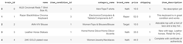
The problem at hand is to predict the prices of any given product, which explains that this is a problem of regression. The features we have in train data are train_id, name, item_condition_id, category_name, brand_name, price, shipping, item_description of the item. We have all the other features in the test data except the price which is our target variable. The features are not only categorical and numerical, but they are also a text description of the item provided by the seller. For example, the text descriptions of the products that are women’s accessories are as follows:
当前的问题是预测任何给定产品的价格,这说明这是回归问题。 我们在火车数据中具有的功能是train_id,名称,item_condition_id,category_name,brand_name,价格,运费,item_description 。 除了价格 (我们的目标变量)外,测试数据中还有其他所有功能。 这些功能不仅是分类功能和数字功能,而且还是卖家提供的商品的文字说明。 例如,作为女士配饰的产品的文本描述如下:

We can see that both are sold at different prices; the first for 16USD and the second for 9USD.
我们可以看到两者以不同的价格出售; 第一个价格为16美元,第二个价格为9美元。
So, the challenge here is that we need to build a model that should predict the right prices for products based on the descriptions as shown in the image above, along with the name of the product, category name, the brand name, the condition of the item, etc.
因此,这里的挑战是我们需要建立一个模型,该模型应该根据上图所示的描述,产品名称,类别名称,品牌名称,使用条件来预测产品的正确价格。物品等
2.误差指标 (2. Error metric)
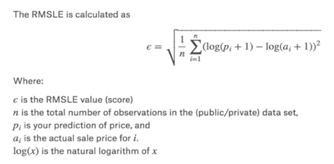
The error metric for this problem is Root Mean Square Logarithmic Error (RMSLE). Please refer to this blog to learn more about the metric. The formula for the metric calculation is shown in the image below:
此问题的误差度量是均方根对数误差(RMSLE)。 请参考此博客以了解有关该指标的更多信息。 下图显示了度量标准的计算公式:
code for calculating RMSLE shown below:
计算RMSLE的代码如下所示:
3.机器学习和深度学习在我们的问题中的应用 (3. Application of Machine Learning and Deep Learning to our problem)
In this era of Artificial Intelligence (AI), the moment we think about AI, the next two buzzwords are Machine learning and Deep learning. We find AI everywhere, indeed they are part and parcel of human life. Be it commuting (e.g. cab booking), medical diagnosis, the personal assistant (e.g. Siri, Alexa), fraud detection, crime detection, online customer support, product recommendations, self-driving cars, and the list goes on. With cutting-edge machine learning and deep-learning algorithms at our disposal, any kind of predictive problem can be solved.
在这个人工智能(AI)时代,我们思考AI的那一刻,接下来的两个流行词是机器学习和深度学习。 我们随处可见AI,的确,它们是人类生活的一部分。 无论是通勤(例如出租车预订),医疗诊断,私人助理(例如Siri,Alexa),欺诈检测,犯罪检测,在线客户支持,产品推荐,自动驾驶汽车,等等。 借助我们提供的最先进的机器学习和深度学习算法,可以解决任何类型的预测问题。
Our problem is unique, as it is a regression task based on NLP (Natural Language Processing). The first step in the NLP is to represent text to number, i.e. to convert the texts into numerical vector representations for the construction of the regressors.
我们的问题是独特的,因为它是基于NLP(自然语言处理)的回归任务。 NLP的第一步是将文本表示为数字,即将文本转换为数字矢量表示形式以构造回归变量。
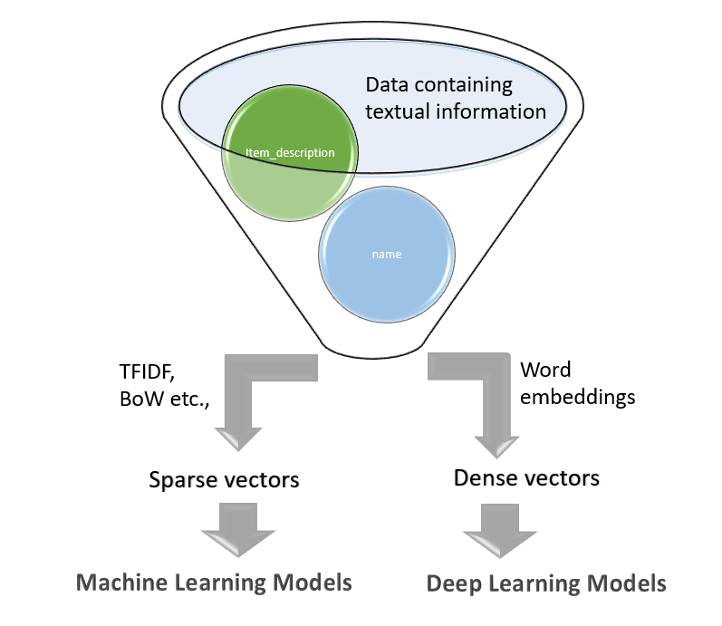
One way to address the price prediction problem is to leverage vectorization techniques such as TF-IDF, BoW, and build fixed-size sparse vector representations that would be used by classic Machine Learning algorithms (e.g. simple linear regressor, tree-based regressor, etc.). The other way is to use Deep NLP architectures (e.g. CNN, LSTM, GRU, or combinations of them) that can learn features on their own and need dense vectors from embedding. In the current analysis, we are investigating both of these approaches.
解决价格预测问题的一种方法是利用TF-IDF,BoW等矢量化技术,并构建固定大小的稀疏矢量表示形式,以供经典的机器学习算法使用(例如,简单的线性回归,基于树的回归等) )。 另一种方法是使用可以自行学习特征并需要嵌入密集向量的Deep NLP架构(例如CNN,LSTM,GRU或它们的组合)。 在当前的分析中,我们正在研究这两种方法。
4.数据来源 (4. Source of Data)
Dataset for this analysis comes from Kaggle, a popular online community or data platform for data scientists.
用于分析的数据集来自Kaggle,它是流行的在线社区或数据科学家的数据平台。

了解数据 (Understanding the data)
The train set consists of over 1.4 million products and the phase 2 test set consists of over 3.4 million products.
训练集包含超过140万种产品,第二阶段测试集包含340万种产品。
Listing the field names in train/test data:
在训练/测试数据中列出字段名称:
train_id or test_id — unique id of the listing
train_id或test_id-列表的唯一ID
name — the product name by the seller. Note that to avoid data leakage the prices in this field are removed and represented as [rm]
名称 -卖方的产品名称。 请注意,为避免数据泄漏,该字段中的价格已删除,并表示为[rm]
item_condition_id — here the seller provides the item conditions
item_condition_id-在此卖家提供商品条件
category_name — category listing for each item
category_name-每个项目的类别列表
brand_name — the corresponding brands which each item belongs to
brand_name-每个项目所属的相应品牌
price — this is our target variable and is represented in USD (column not present in test.tsv)
价格 -这是我们的目标变量,用美元表示(test.tsv中不存在列)
shipping — 1, if the shipping fee is paid by the seller, and 0, otherwise
运费 -1,如果运费由卖方支付,则为0,否则为0
item_description — Each item description is given here and the prices are removed and represented as [rm]
item_description —在此给出每个商品描述,价格被删除并表示为[rm]
A glimpse of the data shown below:
数据如下所示:
5.探索性数据分析-EDA (5. Exploratory Data Analysis — EDA)
EDA, an important step in the Data Science process, is a statistical approach to get more insights from the dataset often using visual methods. Before we plunge into EDA, let’s swiftly look into the data to know more about it. Below is the code snippet to check for null values:
EDA是数据科学过程中的重要步骤,它是一种统计方法,通常使用可视化方法从数据集中获取更多见解。 在涉足EDA之前,让我们快速查看数据以了解更多信息。 下面是检查空值的代码段:
print(train.isnull().sum())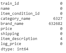
From the above output, we realize that three columns viz., category name, brand name, and item description carry null values. Among them, the brand name includes a lot of missing values (~632k). The column category name includes ~6.3k null values, while the item description has just 4 null values. Let’s deal with them later when we create models, and now we dive into the EDA feature by feature.
从上面的输出中,我们意识到类别名称,品牌名称和项目描述这三列带有空值。 其中,品牌名称包含很多缺失值(〜632k)。 列类别名称包含约6.3k空值,而项目说明仅有4个空值。 让我们稍后在创建模型时进行处理,现在我们逐个功能介绍EDA功能。
5.1 category_name的单变量分析 (5.1 Univariate analysis of category_name)
There are a total of 1287 categories in the training dataset. Shown below is the code snippet for counting:
训练数据集中共有1287个类别。 下面显示的是用于计数的代码段:
category_count = train['category_name'].value_counts()
Plot for the category_count is exhibited below:
下面显示了category_count的图:
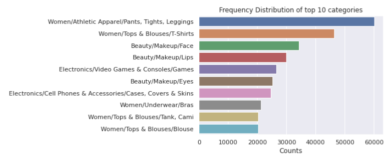
The bar graph above shows the top 10 categories that occur more frequently. One will note that women’s clothing holds the crowning point out of all groups.
上方的条形图显示了发生频率最高的前10个类别。 人们会注意到,女士服装是所有人群中的最高点。
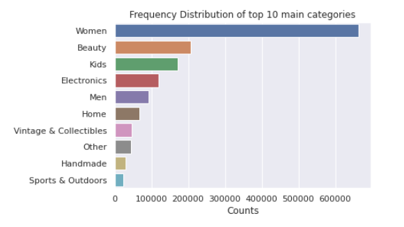
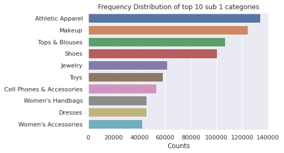
Each category name consists of 3 sub-divisions separated by ‘/’ and has the main-category/sub-category1 / sub-category2 denomination. It is important to separate these and to include them as new features that would allow our model to make better predictions.
每个类别名称均包含3个以'/'分隔的子类别,并具有主类别/子类别1 /子类别2面额。 分离这些并将它们作为新功能包含进来非常重要,这将使我们的模型能够做出更好的预测。
划分类别 (splitting the categories)
We split each category_name as main_category,sub_cat_1,sub_cat_2 in our analysis using the below function.
我们在分析中使用以下函数将每个category_name拆分为main_category , sub_cat_1和sub_cat_2 。
def split_categories(category):
    '''
    function that splits the category column in the dataset and creates 3 new columns:
    'main_category','sub_cat_1','sub_cat_2'
    '''
    try:
      sub_cat_1,sub_cat_2,sub_cat_3 = category.split("/")
      return sub_cat_1,sub_cat_2,sub_cat_3
    except:
      return ("No label","No label","No label")


def create_split_categories(data):
    '''
    function that creates 3 new columns using split_categories function
    : 'main_category','sub_cat_1','sub_cat_2'
    '''
    #https://medium.com/analytics-vidhya/mercari-price-suggestion-challenge-a-machine-learning-regression-case-study-9d776d5293a0
    data['main_category'],data['sub_cat_1'],data['sub_cat_2']=zip(*data['category_name'].\
                                                                  apply(lambda x: split_categories(x)))
Besides, the number of categories in each of the three columns is counted using the code line below:
此外,使用以下代码行计算三列中每列的类别数:
main_category_count_te = test['main_category'].value_counts()
sub_1_count_te = test['sub_cat_1'].value_counts()
sub_2_count_te = test['sub_cat_2'].value_counts()
The above analysis shows that there are 11 main categories which, in turn, are divided into 114 subcategories (subcategory 1) which are further allocated to 865 specific categories (subcategory 2) in train data. The code for plotting the categories is shown below:
以上分析显示,有11个主要类别,依次分为114个子类别(子类别1),这些子类别在火车数据中进一步分配给865个特定类别(子类别2)。 绘制类别的代码如下所示:
def plot_categories(category,title):
  '''
  This function takes in a category and title as input and
  plots the bar chart for the same.
  '''
  #https://seaborn.pydata.org/generated/seaborn.barplot.html
  sns.set(style="darkgrid")
  sns.barplot(x=category[:10].values, y=category[:10].index)
  plt.title(title)
  plt.xlabel('Counts', fontsize=12)
  plt.show()
#https://www.datacamp.com/community/tutorials/categorical-data
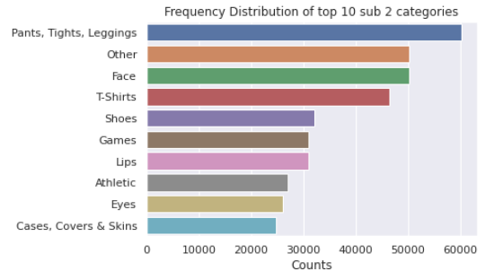
plot_categories(category_count,"Frequency Distribution of top 10 categories")The bar charts of the top 10 items in each column of the category after splitting are included below:
拆分后,类别中每列中前10个项目的条形图包括:
5.2 brand_name的单变量分析 (5.2 Univariate Analysis of brand_name)
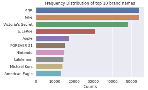
There are a total of 4807 unique brands out of which the top 10 most frequently occurring brands are shown in the bar chart below:
总共有4807个独特品牌,其中以下条形图中显示了最常出现的10个品牌:
plotting code is here:
绘图代码在这里:
#https://www.datacamp.com/community/tutorials/categorical-data
sns.barplot(x=brand_count[:10].values, y=brand_count[:10].index)
plt.title('Frequency Distribution of top 10 brand names')
plt.xlabel('Counts', fontsize=12)
plt.show()
It is noted that the PINK and NIKE brands, followed by Victoria’s Secret, are the ones holding top positions.
值得注意的是,PINK和NIKE品牌紧随其后,位居榜首。
5.3价格的单变量分析 (5.3 Univariate analysis of the price)
Since the price is numerical, we use the describe() function to perceive the statistic summary. Below is the code snippet:
由于价格是数字,因此我们使用describe()函数来感知统计摘要。 下面是代码片段:
train.price.describe()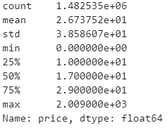
The describe() function explains that the maximum price for any product is $2009 and the minimum price is 0. It is also noted that 75% of the product price range occurs below $29 and 50% of the product price falls below $17, while 25% of the product price falls below $10. The average price range is $26.7.
describe()函数说明,任何产品的最高价格为2009美元,最低价格为0。还应注意,产品价格范围的75%低于29美元,产品价格的50%低于17美元,而25%产品价格的百分比降至10美元以下。 平ASP格范围是26.7美元。
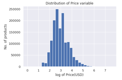
价格变量的分布 (Distribution of price variable)
Plotting the distribution of the target
绘制目标分布
plt.title("Distribution of Price variable")
plt.xlabel("Price(USD)")
plt.ylabel("No. of products")
plt.hist(train['price'],bins=30)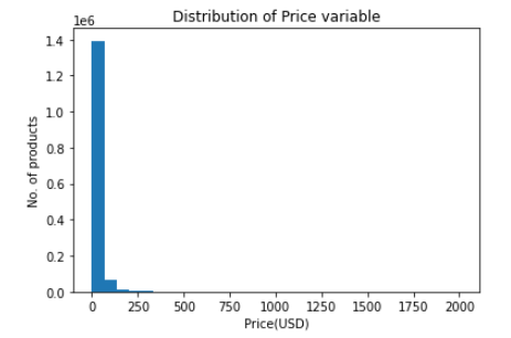
The price feature follows a right-skewed distribution as evident from the above plot. As discussed here, a skewed distribution would result in high Mean Squared Error (MSE) values due to points on the other side of the distribution, and if the data is normally distributed, the MSE is limited. As a result, a log transformation for the price feature is inevitable, and the model can also perform better if the data is normally distributed (see here). This is done with the following code snippet:
从上图可以明显看出, 价格特征遵循右偏分布。 如所讨论的在这里 ,偏态分布将导致高均方误差(MSE)值由于在分配的另一侧的点,并且如果该数据是正态分布时,MSE是有限的。 结果,价格特征的对数转换是不可避免的,并且如果数据是正态分布的,则模型也可以表现更好( 请参见此处 )。 这是通过以下代码片段完成的:
def log_price(price):
    return np.log1p(price)#changes
Shown below is the plot of the price variable after log transformation.
下面显示的是对数转换后的价格变量图。
5.4 item_description的单变量分析 (5.4 Univariate analysis of item_description)
We‘re plotting the word cloud to know the prevailing words in the description. The corresponding code snippet with the plot shown below:
我们正在绘制单词cloud以了解描述中的主要单词。 相应的代码片段,其图如下所示:
word_counter = Counter(train['item_description'])
most_common_words = word_counter.most_common(500)


#https://www.geeksforgeeks.org/generating-word-cloud-python/
# Create and generate a word cloud image:
stopwords = get_stop_words('en')
#https://github.com/Alir3z4/python-stop-words/issues/19
stopwords.extend(['rm'])
wordcloud = WordCloud(stopwords=stopwords,background_color="white").generate(str(most_common_words))


# Display the generated image:
plt.figure(figsize=(10,15))
plt.imshow(wordcloud, interpolation='bilinear')
plt.title("Word cloud generated from the item_descriptions\n")
plt.axis("off")
plt.show()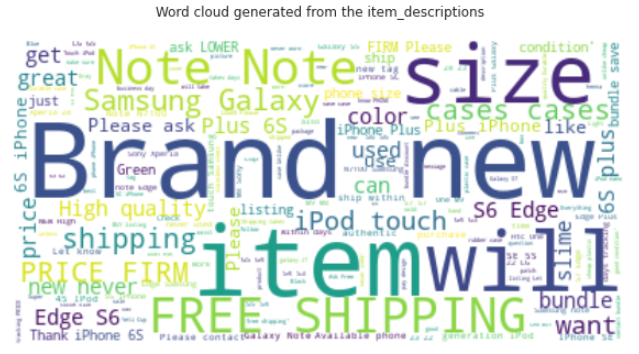
From the word cloud above, one can notice the frequently appearing words in our item_description.
从上面的词云中,您可以注意到我们item_description中经常出现的词。
描述字数 (Wordcount of descriptions)
The text description alone could be an important feature of this problem (refer) i.e. for machine learning models and would help in the process of embedding for deep learning models.
单独的文本描述可能是该问题的一个重要特征( 请参阅参考资料 ),例如对于机器学习模型,这将有助于嵌入深度学习模型。
train['description_wc'] = [len(str(i).split()) for i in train['item_description']]To further investigate the feature, we plot the box plot and the distribution plot shown below along with the code:
为了进一步研究该功能,我们绘制了下面所示的箱形图和分布图以及代码:
箱形图 (Box-plot)
sns.boxplot(train['description_wc'],orient='v')
plt.title("Box plot of description word count")
plt.xlabel("item_description")
plt.ylabel("No. of words")
plt.show()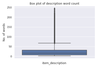
One can notice that the majority descriptions contain approximately less than 40 words.
可以看到,大多数描述都包含大约少于40个字。
密度图 (Density plot)
plt.figure(figsize=(10,3))
sns.distplot(train['description_wc'], hist=False)
plt.title('Plot of the word count for each item description')
plt.xlabel('Number of words in each description')
plt.show()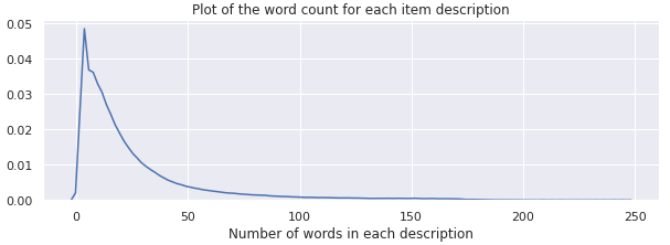
The density plot of the description word count is right-skewed.
描述字数的密度图右偏。
统计摘要 (Summary statistics)
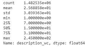
Summary stats indicate that the minimum length of the item_description is 1 while the maximum length is 245. The average length is approximately 25 words. Fewer descriptions are longer, while most of them contain less than 40 words, as we can see in the box-plot.
摘要统计数据表明item_description的最小长度为1,而最大长度为245。平均长度约为25个字。 更少的描述更长,而大多数描述都少于40个字,正如我们在方框图中所看到的那样。
5.5 item_condition_id的单变量分析 (5.5 Univariate analysis of item_condition_id)
The range of the ordinal categorical feature item_condition_id is 1 to 5. Ordinality is that the item with condition 1 is ‘best’ and the item with condition 5 is ‘worst’ (based on this reference). The bar chart of item_condition_id is shown below:
顺序分类特征item_condition_id的范围是1到5。通常是条件1的项目为“最佳”,条件5的项目为“最差”(基于此参考)。 item_condition_id的条形图如下所示:
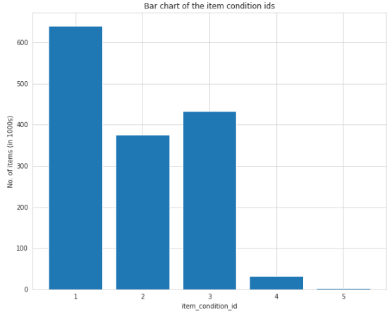
Most items for sale are in good condition as shown in the bar chart above. Consequently, the item with condition 1 is higher, followed by conditions 3 and 2, while the items with conditions 4 and 5 are lower.
如上面的条形图所示,大多数待售物品都处于良好状态。 因此,条件为1的项目较高,其次为条件3和2,而条件为4和5的项目较低。
5.6双变量分析 (5.6 Bivariate analysis)
Knowing the type of association that the target variable possesses with other features would help in the engineering of features. The price variable is therefore compared with two other variables.
知道目标变量与其他特征的关联类型将有助于特征的设计。 因此,将价格变量与其他两个变量进行比较。
价格与运输 (Price Vs Shipping)
As always, plotting would help us to understand things better. The code and the plot are shown below:
与往常一样,绘图将帮助我们更好地理解事物。 代码和图解如下所示:
#https://seaborn.pydata.org/generated/seaborn.boxplot.html


ax = sns.boxplot(x=train['shipping'],y=train['log_price'],palette="Set3",hue=train['shipping'])
handles, _ = ax.get_legend_handles_labels()
ax.legend(handles, ["seller pays", "Buyer pays"])
plt.title('Price distribution', fontsize=15)
plt.show()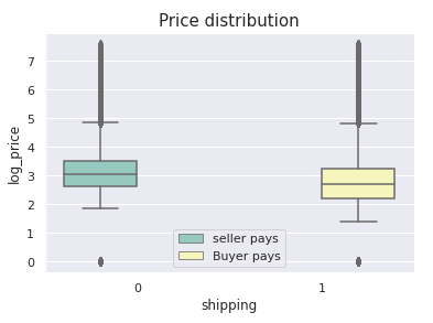
One can observe that when the price of the item is higher, the seller pays for shipping and vice versa.
可以观察到,当商品的价格较高时,卖方将为运费付款,反之亦然。
价格与描述长度 (Price Vs Description length)
The plotting of both variables as we did above.
像上面一样绘制两个变量。
plt.scatter(train['description_wc'],train['price'],alpha=0.4)
plt.title("Price Vs Description length")
plt.xlabel("Description length")
plt.ylabel("Price(USD)")
plt.show()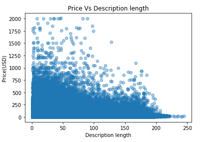
It is remarkable to note that the item with a shorter description length tends to have a higher price than those with longer descriptions.
值得注意的是,描述长度较短的商品往往比描述较长的商品价格更高。
6.现有方法 (6. Existing Approaches)
There are several kernels, blogs, and papers that have made solutions using simple machine learning or deep learning approaches. We are going to brief a few of them:
有几种内核,博客和论文使用简单的机器学习或深度学习方法制定了解决方案。 我们将简要介绍其中的一些:
MLP (MLP)
Pawel and Konstantin have won this competition with their amazing solution. They used a feed-forward neural network-based approach, i.e. a simple MLP that works efficiently on sparse features. Some of the pre-processing tricks performed include one-hot encoding for categorical columns, stemming texts using standard PorterStemmer, BoW-1,2-grams (with/without TF-IDF), concatenation of different fields such as name, brand name and item_description into a single field. They had an exceptional final score of 0.37 (link).
Pawel和Konstantin凭借出色的解决方案赢得了这场比赛。 他们使用了基于前馈神经网络的方法,即简单的MLP,可以有效地处理稀疏特征。 进行的一些预处理技巧包括对分类列进行一键式编码,使用标准PorterStemmer提取文本,BoW-1,2-grams(带/不带TF-IDF), 名称,品牌名称和item_description放入单个字段。 他们获得了非凡的最终得分0.37( 链接 )。
有线电视新闻网 (CNN)
In this study, the author used CNN architecture, along with max-pooling, to vectorize name and item_description separately. He used pre-trained GloVE vectors for word embedding, and embedding is a shared search for both name and item_description. Some useful tricks used are the skip connections of numerical and low cardinality categorical features before the last fully connected layer and the word embeddings’ Average Pooling layer. The author has achieved a striking score of 0.41 from a single deep learning model (link).
在这项研究中,作者使用了CNN架构以及最大池,分别对名称和item_description进行矢量化处理 。 他使用预训练的GloVE向量进行单词嵌入,并且嵌入是对name和item_description的共享搜索。 使用的一些有用技巧是,在最后一个完全连接的层之前,以及数字嵌入的平均池化层之前,跳过数字和低基数分类特征的连接。 作者从单个深度学习模型( 链接 )获得了0.41的惊人分数。
LGBM +山脊 (LGBM + Ridge)
Here, the author has applied a tree-based gradient boosting framework called LightGBM for faster training and higher efficiency. The study also used a simple, faster Ridge model to train. Some featuring techniques include: using CountVectorizer for vectorizing name and category_name columns, TfidfVectorizer for item_description, dummy variables creation for item_condition_id and shipping_id, and LabelBinarizer for brand_name. After the two models were ensembled, the author achieved a score of 0.44. (link)
在这里,作者应用了一个名为LightGBM的基于树的渐变增强框架,以加快训练速度并提高效率。 该研究还使用了简单,快速的Ridge模型进行训练。 一些特色技术包括:使用CountVectorizer矢量化的名字和CATEGORY_NAME列,TfidfVectorizer为ITEM_DESCRIPTION,虚拟变量创作item_condition_id和shipping_id,并LabelBinarizer的BRAND_NAME。 在将两个模型组合在一起后,作者获得了0.44的分数。 ( 链接 )
GRU + 2岭 (GRU + 2 Ridge)
In this study, the author has constructed an associated model using RNN, Ridge, and RidgeCV which yielded an RMSLE of approximately 0.427. Some useful tricks applied here include the use of GRU layers for textual features, scheduled learning decay for RNN training, the use of small batch sizes with 2 epochs, and more than 300k features for Ridge models (link).
在这项研究中,作者使用RNN,Ridge和RidgeCV构建了一个关联模型,得出的RMSLE约为0.427。 这里应用的一些有用技巧包括将GRU图层用于文本特征,用于RNN训练的计划学习衰减,使用具有2个历元的小批量大小以及用于Ridge模型( 链接 )超过300k的特征。
7.数据准备 (7. Data preparation)
数据清理 (Data cleaning)
The minimum price on the Mercari website is $3 based on this reference. Hence in our training data, we keep items whose prices are above $3. Shown below is the code snippet for the same:
根据此参考,Mercari网站上的最低价格为3美元。 因此,在我们的训练数据中,我们保留价格高于3美元的商品。 下面显示的是相同的代码段:
#https://www.kaggle.com/valkling/mercari-rnn-2ridge-models-with-notes-0-42755
train = train.drop(train[(train.price < 3.0)].index)
处理Null / Missing值 (Handling Null/Missing values)
From EDA, we get to know that 3 columns viz., category_name, brand_name, and item_description hold null values. We, therefore, replace them with the appropriate values. We‘re doing this with the following function:
从EDA,我们知道3列,即category_name , brand_name和item_description包含空值。 因此,我们将它们替换为适当的值。 我们使用以下功能进行此操作:
def fill_nan(dataset):
  '''
  Function to fill the NaN values in various columns
  '''
  dataset["item_description"].fillna("No description yet",inplace=True)
  dataset["brand_name"].fillna("missing",inplace=True)
  dataset["category_name"].fillna("missing",inplace=True)
火车测试拆分 (Train-Test Split)
In our analysis, the price field is the target variable ‘y.’ It is important to assess the fitness of our regression models based on the error function, and we need to have ‘y’ observed and ‘y’ predicted. Unfortunately, we do not have the observed target value for evaluating our models. Consequently, the training data is divided into train and test sets.
在我们的分析中, 价格字段是目标变量“ y”。 基于误差函数评估回归模型的适用性很重要,我们需要观察到“ y”并且预测了“ y”。 不幸的是,我们没有用于评估模型的观察目标值。 因此,训练数据分为训练集和测试集。
For the basic linear regression models, the test set consists of 10% of the data, and for deep learning models, the test set includes 20% of the total data.
对于基本线性回归模型,测试集包含10%的数据,对于深度学习模型,测试集包含总数据的20%。
扩展目标 (Scaling the target)
Standardization of the target variable is performed using StandardScaler function from sklearn.preprocessing as shown below:
目标变量的标准化是使用sklearn.preprocessing的StandardScaler函数执行的,如下所示:
global y_scalar
y_scalar = StandardScaler()
y_train = y_scalar.fit_transform(log_price(X_train['price']).values.reshape(-1, 1))
y_test = y_scalar.transform(log_price(X_test['price']).values.reshape(-1, 1))
Since our target variables are standardized using the above function, it is important to scale the predictions back (inverse transform) before we calculate the error metric. This is done by using the following function:
由于我们的目标变量已使用上述函数进行了标准化,因此在计算误差度量之前,将预测值按比例缩小(逆变换)非常重要。 这是通过使用以下功能完成的:
def scale_back(x):
    '''
    Function to inverse transform the scaled values
    '''
    x= np.expm1(y_scalar.inverse_transform(x.reshape(-1,1))[:,0])#changes
    return x
8.型号说明 (8. Model Explanation)
Let us go through the Machine learning and deep learning pipeline in detail.
让我们详细研究机器学习和深度学习管道。
8.1机器学习管道 (8.1 Machine learning pipeline)

In this analysis, Natural Language Processing concepts such as BoW, TFIDF, etc. are used to vectorize texts for machine learning regression models.
在此分析中,自然语言处理概念(例如BoW,TFIDF等)用于对文本进行矢量化以用于机器学习回归模型。
特征构造 (Feature construction)
While performing EDA, we add four new features, i.e., we generate three new columns by splitting the column category, and we add word count of the text description from the item_description. Also, we create one more column based on the length of the name text. So, we’ve got five new features.
在执行EDA时,我们添加了四个新功能,即,通过拆分列类别来生成三个新列,并从item_description添加了文本描述的字数 。 同样,我们根据名称文本的长度再创建一列。 因此,我们有五个新功能。
Our data set consists of categorical features, numeric features, and text features. One must encode the categorical features and vectorize the text features to create a feature matrix that the model uses.
我们的数据集包括分类特征,数字特征和文本特征。 必须对分类特征进行编码并将文本特征向量化,以创建模型使用的特征矩阵。
分类特征编码 (Categorical feature encoding)
We one-hot encode the categorical features such as category_name, main_category,sub_cat_1,sub_cat_2,brand_name using CountVectorizer function from sci-kit learn and encode shipping_id and item_condition_id using get_dummies() function. Below is the code for the same:
我们使用sci-kit的CountVectorizer函数对诸如category_name , main_category , sub_cat_1 , sub_cat_2 , brand_name之类的分类特征进行热编码,并使用get_dummies()函数对shipping_id和item_condition_id进行编码。 下面是相同的代码:
def one_hot_encode(train,test):
    '''
    Function to one hot encode the categorical columns
    '''
    vectorizer = CountVectorizer(token_pattern='.+')

    vectorizer = vectorizer.fit(train['category_name'].values) # fit has to happen only on train data
    column_cat = vectorizer.transform(test['category_name'].values)


    #vectorizing the main_category column
    vectorizer = vectorizer.fit(train['main_category'].values) # fit has to happen only on train data
    column_mc = vectorizer.transform(test['main_category'].values)

    #vectorizing sub_cat_1 column
    vectorizer = vectorizer.fit(train['sub_cat_1'].values) # fit has to happen only on train data
    column_sb1 = vectorizer.transform(test['sub_cat_1'].values)

    #vectorizing sub_cat_2 column
    vectorizer = vectorizer.fit(train['sub_cat_2'].values) # fit has to happen only on train data
    column_sb2 = vectorizer.transform(test['sub_cat_2'].values)


    #vectorizing brand column
    vectorizer = vectorizer.fit(train['brand_name'].astype(str)) # fit has to happen only on train data
    brand_encodes = vectorizer.transform(test['brand_name'].astype(str))

    print("created OHE columns for main_category,sub_cat_1,sub_cat_2\n")
    print(column_cat.shape)
    print(column_mc.shape)
    print(column_sb1.shape)
    print(column_sb2.shape)
    print(brand_encodes.shape)
    print("="*100)
    return column_cat,column_mc,column_sb1,column_sb2,brand_encodes


def get_dummies_item_id_shipping(df):
    df['item_condition_id'] = df["item_condition_id"].astype("category")
    df['shipping'] = df["shipping"].astype("category")
    item_id_shipping = csr_matrix(pd.get_dummies(df[['item_condition_id', 'shipping']],\
                                                      sparse=True).values)
    return item_id_shipping
文字特征向量化 (Text feature vectorizations)
We encode text features name and item_description using BoW (with uni- and bi-grams), and TFIDF(with uni-,bi- and tri-grams) respectively. The function for the same is given below:
我们分别使用BoW(单字和双字)和TFIDF(单字,双字和三字)对文本特征名称和item_description进行编码。 相同的功能如下:
def vectorizer(train,test,column,no_of_features,n_range,vector_type):
    '''
    Function to vectorize text using TFIDF/BoW
    '''
    if str(vector_type) == 'bow':
        vectorizer = CountVectorizer(ngram_range=n_range,max_features=no_of_features).fit(train[column])  #fitting
    else:
        vectorizer = TfidfVectorizer(ngram_range=n_range, max_features=no_of_features).fit(train[column]) # fit has to happen only on train data

    # we use the fitted vectorizer to convert the text to vector
    transformed_text = vectorizer.transform(tqdm(test[column]))
    ###############################
    print("After vectorizations")
    print(transformed_text.shape)
    print("="*100)
    return transformed_text
code using the above function is given below:
使用上述功能的代码如下:
X_train_bow_name = vectorizer(X_train,X_train,'name',100000,(1,2),'bow')
X_test_bow_name = vectorizer(X_train,X_test,'name',100000,(1,2),'bow')
X_train_tfidf_desc = vectorizer(X_train,X_train,'item_description',100000,(1,3),'tfidf')
X_test_tfidf_desc = vectorizer(X_train,X_test,'item_description',100000,(1,3),'tfidf')
特征矩阵 (Feature Matrix)
The final matrix is generated by concatenating all the encoded features (both categorical and text) along with two numerical features, i.e. the word count of the text description and the name. Code for reference below:
通过将所有编码特征(分类特征和文本特征)与两个数字特征(即文本描述的字数和名称)串联在一起,生成最终矩阵。 参考代码如下:
x_train_set = hstack((X_train_bow_name,X_train_tfidf_desc,tr_cat,X_train['wc_name'].values.reshape(-1,1),X_train['wc_desc'].values.reshape(-1,1))).tocsr()
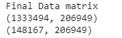
x_test_set = hstack((X_test_bow_name,X_test_tfidf_desc,te_cat,X_test['wc_name'].values.reshape(-1,1),X_test['wc_desc'].values.reshape(-1,1))).tocsr()The resulting final matrix consists of more than 206k features. Indeed, that’s a lot of features.
最终的最终矩阵包含超过206k的特征。 确实,这有很多功能。
初剪模型 (First cut Models)
Choosing an appropriate algorithm for the problem may be a herculean task especially for beginners.
为问题选择合适的算法可能是一项艰巨的任务,特别是对于初学者。
We learn to choose algorithms based on data dimensionality, linearity, training time, type of problem, etc., as discussed here.
我们学习基于数据的维数,线性,培训时间,问题类型等来选择算法,讨论在这里 。
In our analysis, we first experiment with simple linear models such as linear regression, Support Vector Regressor, and for both the models, we choose SGDRegressor from sci-kit learn. Following this, we train Ridge regression.
在我们的分析中,我们首先尝试使用简单的线性模型(例如线性回归,支持向量回归),对于这两个模型,我们都从sci-kit学习中选择SGDRegressor。 之后,我们训练Ridge回归。
We hyperparameter tune the parameters for all the models using GridSearchCV using the following function:
我们使用以下功能使用GridSearchCV对所有模型的参数进行超调:
def hyperparameter_tuning_random(x,y,model_estimator,param_dict,cv_no):
    start = time.time()
    hyper_tuned = GridSearchCV(estimator = model_estimator, param_grid = param_dict,\
                                    return_train_score=True, scoring = 'neg_mean_squared_error',\
                                    cv = cv_no, \
                                    verbose=2, n_jobs = -1)
    hyper_tuned.fit(x,y)
    print("\n######################################################################\n")
    print ('Time taken for hyperparameter tuning is {} sec\n'.format(time.time()-start))
    print('The best parameters_: {}'.format(hyper_tuned.best_params_))
    return hyper_tuned.best_params_
线性回归 (Linear Regression)
Linear regression aims to reduce the error between prediction and actual data. We train simple linear regression using SGDregressor with “squared_loss” and hyperparameter tune for different alphas. The code shown below is the same:
线性回归旨在减少预测数据与实际数据之间的误差。 我们使用带有“ squared_loss”和不同参数的超参数调整的SGDregressor训练简单的线性回归。 下面显示的代码是相同的:
#Hyperparameter tuning
parameters = {'alpha':[10**x for x in range(-10, 7)],
}
model_lr_reg = SGDRegressor(loss = "squared_loss",fit_intercept=False,l1_ratio=0.6)
best_parameters_lr = hyperparameter_tuning_random(x_train_set,y_train,model_lr_reg,parameters,3)
#model with tuned parameters
model_lr_best_param = SGDRegressor(loss = "squared_loss",alpha = best_parameters_lr['alpha'],\
fit_intercept=False)
model_lr_best_param.fit(x_train_set,y_train)
y_train_pred = model_lr_best_param.predict(x_train_set)
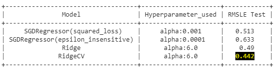
y_test_pred = model_lr_best_param.predict(x_test_set)This simple model yielded an RMSLE of 0.513 for the best alpha = 0.001 on our test data.
对于我们的测试数据,最佳阿尔法= 0.001时,此简单模型的RMSLE为0.513。
支持向量回归: (Support Vector Regressor:)
Support Vector Regressor(SVR) intends to predict the function that deviates from actual data by value no more than epsilon ε(refer). We train an SVR using SGDRegressor with “epsilon_insensitive” as a loss and hyperparameter tune for alphas. This model produced an RMSLE 0.632 for alpha = 0.0001 on our test data. In our case, a simple linear regression performed far better than the support vector machine. Code for SVR is given below:
支持向量回归(SVR)旨在通过不超过ε的值来预测偏离实际数据的函数( 请参阅参考资料)。 我们使用SGDRegressor和“ epsilon_insensitive”作为α的损失和超参数调整来训练SVR。 根据我们的测试数据,该模型在alpha = 0.0001时产生了RMSLE 0.632。 在我们的案例中,简单的线性回归比支持向量机的性能好得多。 SVR的代码如下:
#hyperparameter tuning
parameters_svr = {'alpha':[10**x for x in range(-4, 4)]}
model_svr = SGDRegressor(loss = "epsilon_insensitive",fit_intercept=False)
best_parameters_svr = hyperparameter_tuning_random(x_train_set,y_train,model_svr,parameters_svr,3)


#model with tuned parameters
model_svr_best_param = SGDRegressor(loss = "epsilon_insensitive",alpha = 0.0001,\
                                    fit_intercept=False)
model_svr_best_param.fit(x_train_set,y_train[:,0])
y_train_pred_svr = model_svr_best_param.predict(x_train_set)
y_test_pred_svr = model_svr_best_param.predict(x_test_set)
岭回归 (Ridge Regression)
Ridge regression is next of kin to linear regression with some regularization given by L2-norm to prevent from overfitting. We obtain a good fit using the sci-kit learn Ridge library under the linear-model with an RMSLE of 0.490 for the alpha = 6.0. Below is the code of the Ridge model with hyperparameter tuning:
Ridge回归是线性回归的近亲,并通过L2-范数进行了正则化以防止过度拟合。 使用线性模型下的sci-kit学习Ridge库,对于alpha = 6.0,RMSLE为0.490,我们获得了很好的拟合度。 以下是带有超参数调整的Ridge模型的代码:
#hyperparameter tuning
parameters_ridge = {'alpha':[0.0001,0.001,0.01,0.1,1.0,2.0,4.0,5.0,6.0]}
model_ridge = Ridge(
    solver='auto', fit_intercept=True,
    max_iter=100, normalize=False, tol=0.05, random_state = 1,
)
rs_ridge = hyperparameter_tuning_random(x_train_set,y_train,model_ridge,parameters_ridge,3)


#Model with tuned parameters
ridge_model = Ridge(
    solver='auto', fit_intercept=True,
    max_iter=100, normalize=False, tol=0.05, alpha=6.0,random_state = 1,
)
ridge_model.fit(x_train_set, y_train)
里奇简历 (RidgeCV)
It is a cross-validation estimator that can automatically select the best hyperparameter (refer to: here). In other words, the Ridge regression with built-in cross-validation. As stated in this kernel, that this is performing better than Ridge for our problem, we build the RidgeCV model which yielded an RMSLE of 0.442 for alpha 6.0 on our test data. The code for the same is shown below:
它是一个交叉验证估计器,可以自动选择最佳的超参数(请参阅: 此处 )。 换句话说,带有内置交叉验证的Ridge回归。 如该内核所述,对于我们的问题,此方法的性能优于Ridge,我们建立了RidgeCV模型,该模型在测试数据中得出的alpha 6.0的RMSLE为0.442。 相同的代码如下所示:
from sklearn.linear_model import RidgeCV
print("Fitting Ridge model on training examples...")
ridge_modelCV = RidgeCV(
    fit_intercept=True, alphas=[6.0],
    normalize=False, cv = 2, scoring='neg_mean_squared_error',
)
ridge_modelCV.fit(x_train_set1, y_train)
preds_ridgeCV = ridge_modelCV.predict(x_test_set1)
We can also observe that RidgeCV outperformed in our first cut models. To further improve the score, we are exploring the neural networks that use RNN for this problem.
我们还可以观察到RidgeCV在我们的第一个剪切模型中表现出色。 为了进一步提高分数,我们正在探索使用RNN解决此问题的神经网络。
8.2深度学习管道 (8.2 Deep learning pipeline)
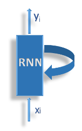
Recurrent Neural Networks(RNN) are good at handling sequence data information(for more information please refer). We use Gated Recurrent Units (GRUs) for building regressors using neural networks, a new type of RNN that is faster to train. From GRU, we obtain text feature vectors for the name, item_description columns after embedding, and for other categorical fields, we use embedding followed by flattening. All of these together form an 80-dimensional feature vector for our deep learning model.
递归神经网络(RNN)擅长处理序列数据信息(有关更多信息,请参阅 )。 我们使用门控递归单元(GRU)通过神经网络构建回归器,该神经网络是一种新型RNN,训练速度更快。 从GRU,我们获得名称,嵌入后的item_description列的文本特征向量,而对于其他类别字段,则使用嵌入后再展平的形式。 所有这些共同构成了我们深度学习模型的80维特征向量。
嵌入 (Embeddings)
Data preparation for the Deep Learning ( DL) pipeline follows the same routine as we do for the ML pipeline except for the train-test split. Here we consider 20% of the training data to be test data. As mentioned earlier, the DL pipeline requires dense vectors, and neural network embedding is an efficient means of representing our discrete variables as continuous vectors (refer).
深度学习(DL)管道的数据准备遵循与ML管道相同的例程,除了训练测试拆分。 在这里,我们将20%的训练数据视为测试数据。 如前所述,DL流水线需要密集的向量,而神经网络嵌入是将离散变量表示为连续向量的有效方法( 请参阅参考资料 )。
标记化和填充 (Tokenization and Padding)
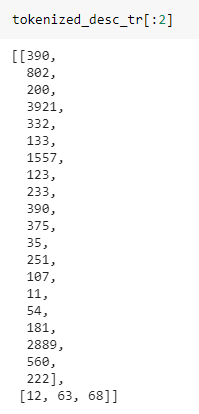
The Embedding Layer requires the input to be integer encoded(refer). As a result, we encode text data using the Tokenizer API, and here is the code snippet for the same:
嵌入层要求输入是整数编码的( 请参阅参考资料 )。 结果,我们使用Tokenizer API对文本数据进行编码,以下是相同的代码段:
def tokenize_text(train,test,column):
    #AAIC course reference
    global t
    t = Tokenizer()
    t.fit_on_texts(train[column].str.lower())
    vocab_size = len(t.word_index) + 1
    # integer encode the documents
    encoded_text_tr = t.texts_to_sequences(train[column].str.lower())
    encoded_text_te = t.texts_to_sequences(test[column].str.lower())
    return encoded_text_tr,encoded_text_te,vocab_size
Screenshot of sample description data after tokenization is shown below:
标记化后的示例描述数据的屏幕截图如下:
Following tokenization, we pad the sequences. The name and description texts are of different lengths and Keras prefers input sequences to be of the same length. We calculate the percentage of data points that fall above a specific range of words to determine the length of the padding.
在标记化之后,我们填充序列。 名称和描述文本的长度不同,Keras希望输入序列的长度相同。 我们计算落入特定单词范围内的数据点的百分比,以确定填充的长度。
Code is shown below for selecting the padding length for description text:
下面显示的代码用于选择描述文本的填充长度:
print("% of sequence containing len > 160 is")
len(X_train[X_train.wc_desc > 160])/X_train.shape[0]*100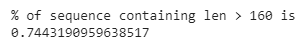
From the image above we see the percentage of points whose length is above 160 is 0.7 which is < 1%. Hence we pad description text with 160. Similarly, we calculate for the name column and we go for 10. The corresponding code snippet is shown below:
从上图可以看到,长度超过160的点的百分比为0.7,即<1%。 因此,我们用160填充描述文本。类似地,我们为name列计算,然后为10。相应的代码段如下所示:
print("% of name containing len > 10 is")
len(X_train[X_train.wc_name > 10])/X_train.shape[0]*100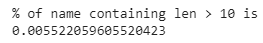
Further, we encode the categorical variables based on ranking and the code snippet is shown below:
此外,我们根据排名对分类变量进行编码,代码段如下所示:
def rank_category(dataset,column_name):
    '''This function takes a column name which is categorical and returns the categories with rank'''
    counter = dataset[column_name].value_counts().index.values
    total = list(dataset[column_name])
    ranked_cat = {}
    for i in range(1,len(counter)+1):
        ranked_cat.update({counter[i-1] : i})
    return ranked_cat,len(counter)


def encode_ranked_category(train,test,column):
    '''
    This function calls the rank_category function and returns the encoded category column    '''
    train[column] = train[column].astype('category')
    test[column] = test[column].astype('category')

    cat_list = list(train[column].unique())
    ranked_cat_tr,count = rank_category(train,column)


    encoded_col_tr = []
    encoded_col_te = []


    for category in train[column]:
        encoded_col_tr.append(ranked_cat_tr[category])


    for category in test[column]:
        if category in cat_list:
            encoded_col_te.append(ranked_cat_tr[category])
        else:
            encoded_col_te.append(0)

    encoded_col_tr = np.asarray(encoded_col_tr)
    encoded_col_te = np.asarray(encoded_col_te)
    return encoded_col_tr,encoded_col_te,count
Note: All the embeddings are learned along with the model itself.
注意:所有嵌入都与模型本身一起学习。
The entire data preparation pipeline, along with encoding, tokenizing, and padding is performed by the following function:
整个数据准备管道以及编码,标记和填充均由以下功能执行:
def data_gru(train,test):
global max_length,desc_size,name_size
encoded_brand_tr,encoded_brand_te,brand_len = encode_ranked_category(train,test,'brand_name')
encoded_main_cat_tr,encoded_main_cat_te,main_cat_len = encode_ranked_category(train,test,'main_category')
encoded_sub_cat_1_tr,encoded_sub_cat_1_te,sub_cat1_len = encode_ranked_category(train,test,'sub_cat_1')
encoded_sub_cat_2_tr,encoded_sub_cat_2_te,sub_cat2_len = encode_ranked_category(train,test,'sub_cat_2')
tokenized_desc_tr,tokenized_desc_te,desc_size = tokenize_text(train,test,'item_description')
tokenized_name_tr,tokenized_name_te,name_size = tokenize_text(train,test,'name')
max_length = 160
desc_tr_padded = pad_sequences(tokenized_desc_tr, maxlen=max_length, padding='post')
desc_te_padded = pad_sequences(tokenized_desc_te, maxlen=max_length, padding='post')
del tokenized_desc_tr,tokenized_desc_te
name_tr_padded = pad_sequences(tokenized_name_tr, maxlen=10, padding='post')
name_te_padded = pad_sequences(tokenized_name_te, maxlen=10, padding='post')
del tokenized_name_tr,tokenized_name_te
gc.collect()
train_inputs = [name_tr_padded,desc_tr_padded,encoded_brand_tr.reshape(-1,1),\
encoded_main_cat_tr.reshape(-1,1),encoded_sub_cat_1_tr.reshape(-1,1),\
encoded_sub_cat_2_tr.reshape(-1,1),train['shipping'],\
train['item_condition_id'],train['wc_desc'],\
train['wc_name']]
test_inputs = [name_te_padded,desc_te_padded,encoded_brand_te.reshape(-1,1),\
encoded_main_cat_te.reshape(-1,1),encoded_sub_cat_1_te.reshape(-1,1),\
encoded_sub_cat_2_te.reshape(-1,1),test['shipping'],\
test['item_condition_id'],test['wc_desc'],\
test['wc_name']]
item_condition_counter = train['item_condition_id'].value_counts().index.values
list_var = [brand_len,main_cat_len,sub_cat1_len,sub_cat2_len,len(item_condition_counter)]
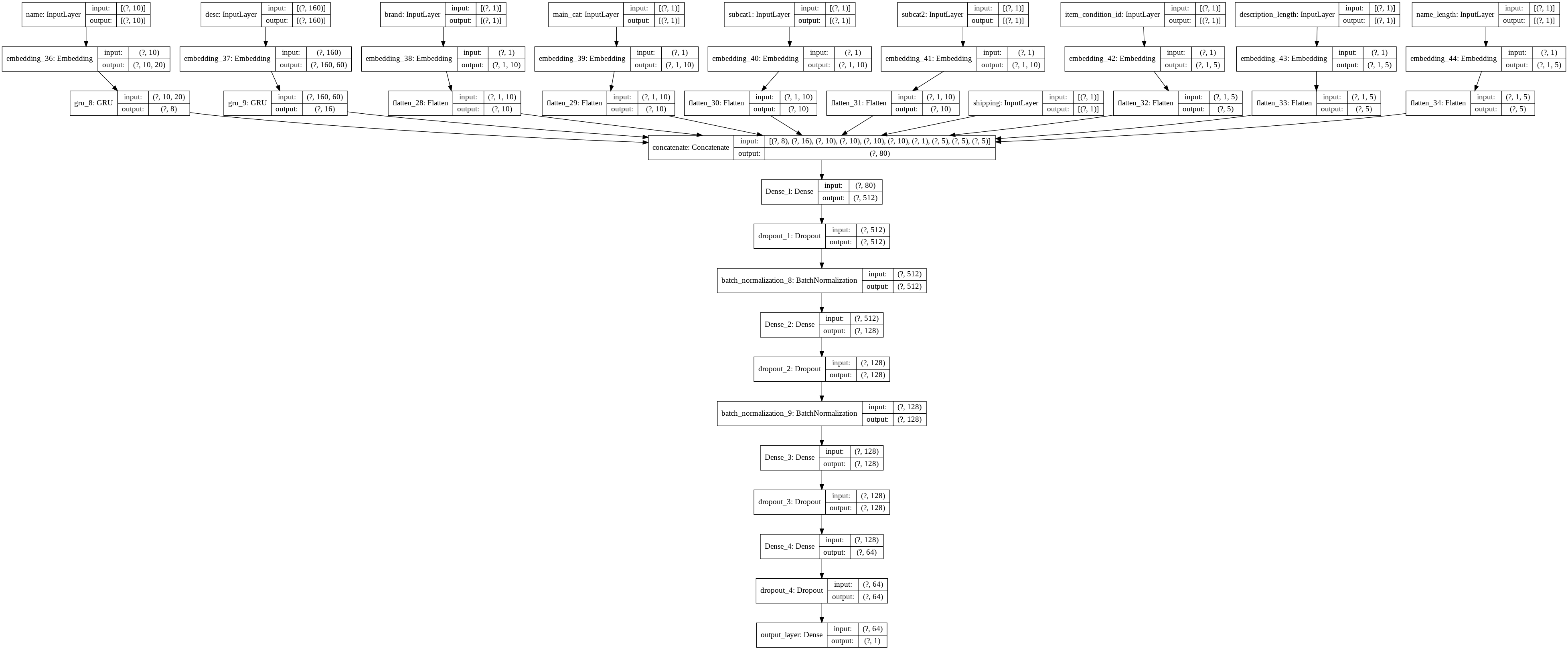
return train_inputs,test_inputs,list_var网络架构 (Network architecture)
Network design for the current analysis is inspired by this kernel. Besides, we experiment with extra drop out layers and batch-normalization layers in this framework. Below is the code snippet for building our network:
网络设计当前分析的灵感来自这个内核。 此外,我们在此框架中尝试了额外的退出层和批处理规范化层。 以下是用于构建我们的网络的代码段:
def construct_GRU(train,var_list,drop_out_list):
    #GRU input layer for name
    input_name =  tf.keras.layers.Input(shape=(10,), name='name')
    embedding_name = tf.keras.layers.Embedding(name_size, 20)(input_name)
    gru_name = tf.keras.layers.GRU(8)(embedding_name)

    #GRU input layer for description
    input_desc =  tf.keras.layers.Input(shape=(max_length,), name='desc')
    embedding_desc = tf.keras.layers.Embedding(desc_size, 60)(input_desc)
    gru_desc = tf.keras.layers.GRU(16)(embedding_desc)


    #input layer for brand_name
    input_brand =  tf.keras.layers.Input(shape=(1,), name='brand')
    embedding_brand = tf.keras.layers.Embedding(var_list[0] + 1, 10)(input_brand)
    flatten1 = tf.keras.layers.Flatten()(embedding_brand)


    #categorical input layer main_category
    input_cat = tf.keras.layers.Input(shape=(1,), name='main_cat')
    Embed_cat = tf.keras.layers.Embedding(var_list[1] + 1, \
                                          10,input_length=1)(input_cat)
    flatten2 = tf.keras.layers.Flatten()(Embed_cat)


    #categorical input layer sub_cat_1
    input_subcat1 = tf.keras.layers.Input(shape=(1,), name='subcat1')
    Embed_subcat1 = tf.keras.layers.Embedding(var_list[2] + 1, \
                                              10,input_length=1)(input_subcat1)
    flatten3 = tf.keras.layers.Flatten()(Embed_subcat1)


    #categorical input layer sub_cat_2
    input_subcat2 = tf.keras.layers.Input(shape=(1,), name='subcat2')
    Embed_subcat2 = tf.keras.layers.Embedding(var_list[3] + 1, \
                                              10,input_length=1)(input_subcat2)
    flatten4 = tf.keras.layers.Flatten()(Embed_subcat2)


    #categorical input layer shipping
    input_shipping = tf.keras.layers.Input(shape=(1,), name='shipping')

    #categorical input layer item_condition_id
    input_item = tf.keras.layers.Input(shape=(1,), name='item_condition_id')
    Embed_item = tf.keras.layers.Embedding(var_list[4] + 1, \
                                           5,input_length=1)(input_item)
    flatten5 = tf.keras.layers.Flatten()(Embed_item)


    #numerical input layer
    desc_len_input = tf.keras.layers.Input(shape=(1,), name='description_length')
    desc_len_embd = tf.keras.layers.Embedding(DESC_LEN,5)(desc_len_input)
    flatten6 = tf.keras.layers.Flatten()(desc_len_embd)


    #name_len input layer
    name_len_input = tf.keras.layers.Input(shape=(1,), name='name_length')
    name_len_embd = tf.keras.layers.Embedding(NAME_LEN,5)(name_len_input)
    flatten7 = tf.keras.layers.Flatten()(name_len_embd)


    # concatenating the outputs
    concat_layer = tf.keras.layers.concatenate(inputs=[gru_name,gru_desc,flatten1,flatten2,flatten3,flatten4,input_shipping,flatten5,\
                                                       flatten6,flatten7],name="concatenate")
    #dense layers
    Dense_layer1 = tf.keras.layers.Dense(units=512,activation='relu',kernel_initializer='he_normal',\
                                         name="Dense_l")(concat_layer)
    dropout_1 = tf.keras.layers.Dropout(drop_out_list[0],name='dropout_1')(Dense_layer1)
    batch_n1 = tf.keras.layers.BatchNormalization()(dropout_1)

    Dense_layer2 = tf.keras.layers.Dense(units=128,activation='relu',kernel_initializer='he_normal',\
                                         name="Dense_2")(batch_n1)
    dropout_2 = tf.keras.layers.Dropout(drop_out_list[1],name='dropout_2')(Dense_layer2)
    batch_n2 = tf.keras.layers.BatchNormalization()(dropout_2)


    Dense_layer3 = tf.keras.layers.Dense(units=128,activation='relu',kernel_initializer='he_normal',\
                                         name="Dense_3")(batch_n2)
    dropout_3 = tf.keras.layers.Dropout(drop_out_list[2],name='dropout_3')(Dense_layer3)


    Dense_layer4 = tf.keras.layers.Dense(units=64,activation='relu',kernel_initializer='he_normal',\
                                         name="Dense_4")(dropout_3)
    dropout_4 = tf.keras.layers.Dropout(drop_out_list[3],name='dropout_4')(Dense_layer4)

    #output_layer
    final_output = tf.keras.layers.Dense(units=1,activation='linear',name='output_layer')(dropout_4)


    model = tf.keras.Model(inputs=[input_name,input_desc,input_brand,input_cat,input_subcat1,input_subcat2,\
                                   input_shipping,input_item,desc_len_input,name_len_input],
                           outputs=[final_output])
    # we specified the model input and output
    print(model.summary())
    img_path = "GRU_model_2_lr.png"
    plot_model(model, to_file=img_path, show_shapes=True, show_layer_names=True)
    return model
Take a look at our network below:
在下面查看我们的网络:
深度学习模型 (Deep Learning Models)
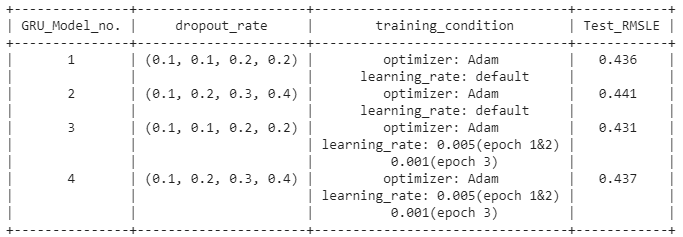
A total of four models are trained that differ in their drop-out and learning-rate. Each network consists of four drop-out layers, and for each of these layers, we try different drop-out rates for all models (see the results for details).
总共训练了四个模型,这些模型的辍学率和学习率不同。 每个网络都由四个退出层组成,对于这些层中的每一个,我们对所有模型尝试不同的退出率(有关详细信息,请参见结果)。
训练 (Training)
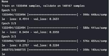
For training Model 1 and Model 2, we use Adam optimizer with the default learning rate. Further, these models are trained for 3 epochs with doubling batch-size. The RMSLE on our test data for Model 1 & 2 is 0.436 and 0.441, respectively. The model training is illustrated below:
对于训练模型1和模型2,我们使用具有默认学习率的Adam优化器。 此外,将这些模型训练了3个时期,批次大小增加了一倍。 模型1和2的测试数据的RMSLE分别为0.436和0.441。 模型训练如下图所示:
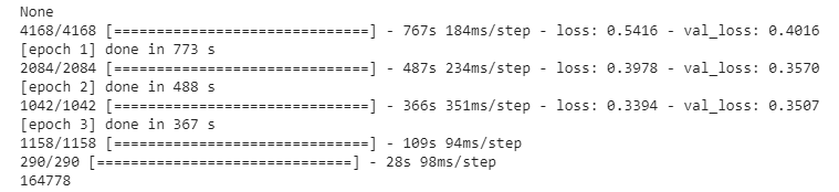
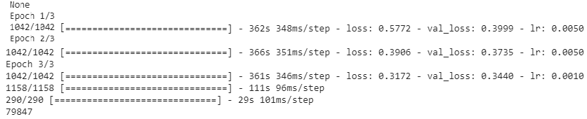
Model 3 & 4 are trained using Adam optimizer with scheduled learning rate. Totally 3 epochs with batch-size of 1024. For epoch 1 & 2, the learning rate is 0.005, and we reduce it to 0.001 for the final epoch. The training for Model 4 is presented below:
使用计划的学习率的Adam优化器训练模型3和模型4。 总共3个纪元,批处理大小为1024。对于纪元1和2,学习率是0.005,对于最后一个纪元,我们将其降低到0.001。 下面介绍了模型4的培训:
模型平均组装 (Model average Ensembling)
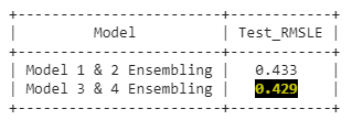
Model averaging is an ensemble learning technique to reduce high variance in neural networks. In the present analysis, we ensemble models that are trained under conditions that differ in their drop-out regularization(refer). Each model takes about 30 to 35 minutes to train. Considering the training time, we only include two models for ensembling. Thus, out of four models, two ensembles are created, i.e, one from Model 1 & 2 that achieves an RMSLE 0.433 and the other from Model 3 & 4 with an RMSLE 0.429
模型平均是减少神经网络中高方差的整体学习技术。 在当前的分析中,我们集成了在辍学正则化不同的条件下训练的模型( 请参阅参考资料 )。 每个模型大约需要30到35分钟的训练时间。 考虑到训练时间,我们只包括两个模型。 因此,在四个模型中,创建了两个合奏,即一个来自模型1和2的RMSLE 0.433,另一个来自模型3和4的RMSLE 0.429
The code for ensembling Model 1 & 2 is shown below:
组合模型1和2的代码如下所示:
#https://machinelearningmastery.com/model-averaging-ensemble-for-deep-learning-neural-networks/
y_hats = np.array([preds_m1_te,te_preds_m2]) #making an array out of all the predictions
# mean across ensembles
mean_preds = np.mean(y_hats, axis=0)
print("RMSLE on test: {}".format(rmsle_compute(X_test['price'],scale_back(mean_preds))))
We observe that the ensemble from Model 3 & 4 outperforms in our train-test split data.
我们观察到,从模型3和4个性能优于我们的列车测试数据分割的整体 。
最终模型 (Final Models)
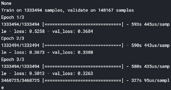
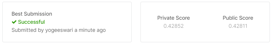
To achieve the final score from Kaggle, we now train in Kaggle kernel. We build two models identical to Model 3 & 4 for ensembling. Exhibited below is the screenshot of the models trained in Kaggle:
为了获得Kaggle的最终成绩,我们现在使用Kaggle内核进行训练。 我们构建了两个与模型3和4相同的模型进行集成。 下面展示的是在Kaggle中训练的模型的屏幕截图:
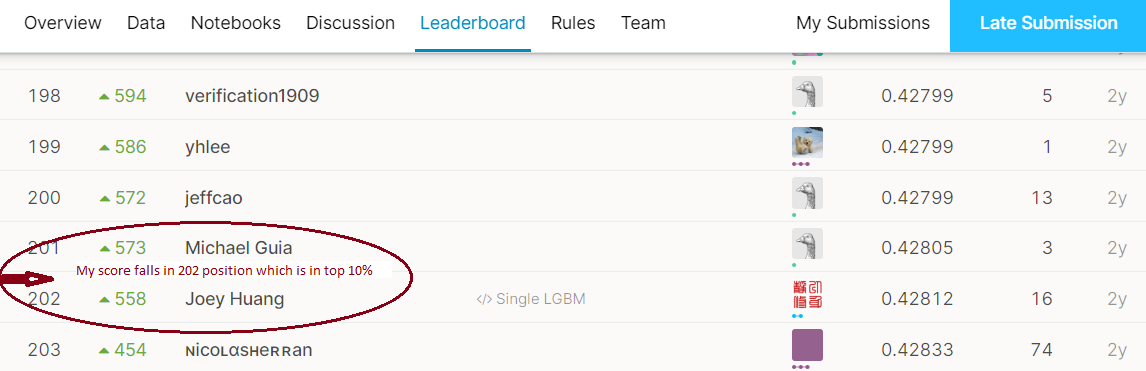
Model average ensembling for these two models yields 0.428 in Kaggle public score on our final test data containing ~3.4 million products. Thus, we accomplish a score that is in the top 10% of the leader board.
在包含约340万种产品的最终测试数据上,这两个模型的模型平均集成在Kaggle公众评分中为0.428 。 因此,我们所获得的分数在排行榜中排名前10% 。
9.结果 (9. Results)
Shown below is a summary screenshot of the outputs of the model:
下面显示的是模型输出的摘要屏幕截图:
The output from the Machine Learning pipeline:
机器学习管道的输出:
Output snapshot from Deep Learning pipeline:
深度学习管道的输出快照:
Screenshot of Ensembling output:
集成输出的屏幕截图 :
Kaggle submission score:
Kaggle提交分数 :
10.我尝试改善RMSLE (10. My attempts to improve RMSLE)
Generally, the kernels of Kaggle ‘s competitors are didactic sources. The present analysis is inspired by this, this one and some from the winner solution. The strategies that have improved our score are as follows:
通常,Kaggle竞争对手的内核是有说服力的。 本分析的灵感源于这一点 , 这一点和一些来自获奖者解决方案。 提高我们分数的策略如下:
Including stopwords for analysis: One key to this problem is that removing the stopwords in the text description/name affects the RMSLE score. The retention of stopwords improves the score.
包括停用词以供分析:解决此问题的一个关键是删除文本描述/名称中的停用词会影响RMSLE分数。 保留停用词可以提高得分。
Considering more text features for model building: In total, we get 206k features which include 200k features from textual data alone. Giving more importance to textual information in this problem improves the score.
考虑用于模型构建的更多文本特征:总共,我们获得了206k的特征,其中仅文本数据就包含了200k的特征。 在此问题中更加重视文本信息可提高得分。
Bi-grams and Tri-grams: In NLP, it is customary to include n-grams such as bi-gram, tri-gram, etc. if we intend to add some semantics during vectorization. In our study, we apply uni- and bi-grams using Bag of Words for name and uni-, bi- & tri-grams for item_description using TFIDF.
Bi-gram和Tri-grams:在NLP中,如果我们打算在向量化过程中添加一些语义,通常会包含n-grams,例如bi-gram,Tri-gram等。 在我们的研究中,我们应用使用字姓名和单向的包单向和双向克,双和三克ITEM_DESCRIPTION使用TFIDF。
Filtering data based on price: Mercari does not allow to post items that are less than $3. Thus, those rows whose product price is less than $3 would be erroneous points. Removing them would help the model to perform better.
根据价格过滤数据 :Mercari不允许发布价格低于3美元的商品。 因此,那些产品价格低于$ 3的行将是错误的点。 删除它们将有助于模型更好地执行。
Model training with small batch-size & few epochs: using a batch-size of 1024 with scheduled learning improved the score
以小批量和少时期进行模型训练:使用1024的批量进行计划学习可提高得分
Ensembling two neural network models: this strategy is exclusive to the current study, which has pushed the score higher on the leader board. We performed our predictive analysis by training two neural network models and building their ensemble.
整合了两个神经网络模型:该策略是当前研究的专有技术,这使排行榜上的得分更高。 我们通过训练两个神经网络模型并建立整体来执行我们的预测分析。
11.今后的工作 (11. Future work)
It is possible to improve the score by exploring the following options:
通过探索以下选项,可以提高分数:
- using Multilayer perceptrons as it is a popular one for this problem 使用多层感知器,因为它是解决此问题的一种流行方法
- using CNN in combination with RNN for processing text data 将CNN与RNN结合使用以处理文本数据
- adding more GRU layers or fine-tuning further 添加更多的GRU层或进一步微调
These are some of the possibilities we would like to explore subsequently.
这些是我们随后希望探索的一些可能性。


 973
973


 被折叠的 条评论
为什么被折叠?
被折叠的 条评论
为什么被折叠?
 到【灌水乐园】发言


