机器学习和深度学习的模型_机器学习和深度学习模型的网格搜索

最新推荐文章于 2024-08-08 20:45:00 发布

weixin_26737625

最新推荐文章于 2024-08-08 20:45:00 发布

阅读量534

点赞数

文章标签：机器学习深度学习人工智能 python tensorflow

原文链接：https://medium.com/datadriveninvestor/grid-search-for-ml-deep-learning-models-260d07541b18

版权

本文探讨了如何在机器学习和深度学习模型中使用网格搜索技术进行参数调优，以提高模型的性能。通过翻译自DataDrivenInvestor的文章，详细解释了在Python环境中，特别是在TensorFlow框架下实施这一过程的方法。

摘要由CSDN通过智能技术生成

机器学习和深度学习的模型

Full guide to grid search on finding the best hyper parameters for our regular ml models to deep learning models

有关为常规ml模型到深度学习模型找到最佳超级参数的网格搜索的完整指南

Hi how are you doing, I hope its great.

嗨，你好吗，我希望它很棒。

Today we will look into ways to find the best parameters for our Machine Learning models as well as for our Deep Learning models. Finding the best parameters by manual tuning is tedious process and time consuming as it contains so many parameters to be test over and over again. Well it’s a time consuming and not productive. So to overcome this issue we will look into a method ‘GRID SEARCH’ to automate the task of finding the best model parameters for us.

今天，我们将研究为我们的机器学习模型和深度学习模型找到最佳参数的方法。通过手动调整查找最佳参数是繁琐的过程和耗时的工作，因为它包含许多参数，需要一遍又一遍地进行测试。嗯，这很耗时，而且没有生产力。因此，为了克服这个问题，我们将研究一种“ GRID SEARCH”方法，以自动执行为我们找到最佳模型参数的任务。

We will divide this into 2 section: a) Grid Search for finding the best hyper-parameters for our machine learning model b.) Grid Search for Deep Learning models.

我们将其分为两部分： a)网格搜索，为我们的机器学习模型找到最佳的超参数b。)网格搜索，用于深度学习模型。

Let’s start with a) Grid Search for machine learning models

让我们从a)开始进行机器学习模型的网格搜索

For this example we will use a data that can be used for credit scoring. In this dataset we have details like income, age, loan and defaulter in 1-yes or 0-no. Let’s first make our simple machine learning model to predict whether we should approve for credit or not.

在此示例中，我们将使用可用于信用评分的数据。在此数据集中，我们有详细信息，例如收入，年龄，贷款和违约者(以1是或0是)。首先，让我们建立简单的机器学习模型，以预测我们是否应该批准学分。

#Importing the libraries
import numpy as np
import matplotlib.pyplot as plt
import pandas as pd#Importing the dataset
dataset = pd.read_csv('credit_data.csv', sep=",")#drop the missing values
dataset = dataset.dropna()
X = dataset.iloc[:,1:4].values
y = dataset.iloc[:, 4].values

First we load the data and define the X-dependent variables( 0 -3rd column) and y-independent variable(defaulter 4th column)

首先，我们加载数据并定义X相关变量(0 -3列)和y独立变量(默认为第4列)

#----------------------------------------------------------#Splitting the dataset into the Training set and Test set
from sklearn.model_selection import train_test_split
X_train, X_test, y_train, y_test = train_test_split(X, y, test_size = 0.25, random_state = 0)from sklearn.preprocessing import StandardScaler
sc = StandardScaler()
X_train = sc.fit_transform(X_train)
X_test = sc.transform(X_test)#Fitting SVM to the Training setfrom sklearn.svm import SVC
svm_model = SVC(kernel = 'linear', random_state = 0)
svm_model.fit(X_train, y_train)#Predicting the Test set results
y_pred = svm_model.predict(X_test)#We can also compare the actual versus predicted
df = pd.DataFrame({'Actual': y_test.flatten(), 'Predicted': y_pred.flatten()})
df#Making the Confusion Matrix
from sklearn.metrics import confusion_matrix
cm = confusion_matrix(y_test, y_pred)#evaluation Metrics
from sklearn import metrics
print('Accuracy Score:', metrics.accuracy_score(y_test, y_pred))
print('Balanced Accuracy Score:', metrics.balanced_accuracy_score(y_test, y_pred))
print('Average Precision:',metrics.average_precision_score(y_test, y_pred))

Then we will split the data into train and test, scale our data before we fit our model. For these example we will use Support Vector Machine (SVM) which is one of the powerful classifier with default parameters.

然后，在将数据拟合到模型之前，我们会将其分为训练和测试，缩放数据。对于这些示例，我们将使用支持向量机(SVM)，它是具有默认参数的强大分类器之一。

With evaluation Metrics of the model we get

通过模型的评估指标，我们得到

Accuracy Score: 0.948
Balanced Accuracy Score: 0.8707788671023965
Average Precision: 0.6733662239089184

It’s time to use the Grid Search to automate the search of best parameters of our svm_model.

现在是时候使用“网格搜索”来自动搜索svm_model的最佳参数了。

#Applying k-Fold Cross Validationfrom sklearn.model_selection import cross_val_score
accuracies = cross_val_score(estimator = svm_model, X = X_train, y = y_train, cv = 10)
accuracies.mean()
accuracies.std()#Applying Grid Search to find the best model and the best parametersfrom sklearn.model_selection import GridSearchCVparameters = [{'C': [1, 10, 100, 1000], 'kernel': ['linear']},{'C': [1, 10, 100, 1000], 'kernel': ['rbf'], 'gamma': [0.1, 0.2, 0.3, 0.4, 0.5, 0.6, 0.7, 0.8, 0.9]}]grid_search = GridSearchCV(estimator = svm_model,param_grid = parameters,scoring = 'accuracy',cv = 10)grid_search = grid_search.fit(X_train, y_train)best_accuracy = grid_search.best_score_
best_parameters = grid_search.best_params_

Well what we got here is pretty much creating a list of parameters and feed it into GridSearch with cross validation cv= 10 and we have

好吧，我们在这里得到的几乎是创建一个参数列表，并通过交叉验证cv = 10将其输入到GridSearch中，

best_parameters
Out[165]: {'C': 1000, 'gamma': 0.9, 'kernel': 'rbf'}best_accuracy
Out[166]: 0.9953243847874722

Alright! Let’s see if these Hyper-parameters can improve the accuracy of our model.

好的！让我们看看这些超参数是否可以提高模型的准确性。

#Fitting SVM to the Training setfrom sklearn.svm import SVC
svm_model = SVC(kernel = 'rbf', C = 1000, gamma = 0.9, random_state = 0)svm_model.fit(X_train, y_train)#Predicting the Test set results
y_pred = svm_model.predict(X_test)#We can also compare the actual versus predicted
df = pd.DataFrame({'Actual': y_test.flatten(), 'Predicted': y_pred.flatten()})
df#Making the Confusion Matrix
from sklearn.metrics import confusion_matrix
cm = confusion_matrix(y_test, y_pred)#evaluation Metrics
from sklearn import metrics
print('Accuracy Score:', metrics.accuracy_score(y_test, y_pred))
print('Balanced Accuracy Score:', metrics.balanced_accuracy_score(y_test, y_pred))
print('Average Precision:',metrics.average_precision_score(y_test, y_pred))Accuracy Score: 0.994
Balanced Accuracy Score: 0.9903322440087146
Average Precision: 0.9587348678601876

Nice! It did improved from 0.94 to 0.99. You can use these code as a template with few modifications like the list of parameters for different types of classifiers and to know the of parameters you can simply select the classifier name ‘svm’ + press ‘ctrl’ + ‘i’

真好！确实从0.94提高到0.99 。您可以将这些代码用作模板，并进行一些修改，例如针对不同类型的分类器的参数列表，并且要了解参数的种类，您只需选择分类器名称'svm'+按'ctrl'+'i'

Let’s me put all of the pieces together.

让我将所有片段放在一起。

#Importing the libraries
import numpy as np
import matplotlib.pyplot as plt
import pandas as pd#Importing the dataset
dataset = pd.read_csv('credit_data.csv', sep=",")#drop the missing values
dataset = dataset.dropna()X = dataset.iloc[:,1:4].values
y = dataset.iloc[:, 4].values#---------------------------------------------------------
#Splitting the dataset into the Training set and Test set
from sklearn.model_selection import train_test_split
X_train, X_test, y_train, y_test = train_test_split(X, y, test_size = 0.25, random_state = 0)from sklearn.preprocessing import StandardScaler
sc = StandardScaler()
X_train = sc.fit_transform(X_train)
X_test = sc.transform(X_test)#Fitting SVM to the Training set
from sklearn.svm import SVC
svm_model = SVC(kernel = 'linear', random_state = 0)
svm_model.fit(X_train, y_train)#Predicting the Test set results
y_pred = svm_model.predict(X_test)#We can also compare the actual versus predicted
df = pd.DataFrame({'Actual': y_test.flatten(), 'Predicted': y_pred.flatten()})
df#Making the Confusion Matrix
from sklearn.metrics import confusion_matrix
cm = confusion_matrix(y_test, y_pred)#evaluation Metrics 
from sklearn import metrics
print('Accuracy Score:', metrics.accuracy_score(y_test, y_pred))  
print('Balanced Accuracy Score:', metrics.balanced_accuracy_score(y_test, y_pred)) 
print('Average Precision:',metrics.average_precision_score(y_test, y_pred))##########################################################Applying k-Fold Cross Validation
from sklearn.model_selection import cross_val_score
accuracies = cross_val_score(estimator = svm_model, X = X_train, y = y_train, cv = 10)
accuracies.mean()
accuracies.std()#Applying Grid Search to find the best model and the best parameters
from sklearn.model_selection import GridSearchCV
parameters = [{'C': [1, 10, 100, 1000], 'kernel': ['linear']},
              {'C': [1, 10, 100, 1000], 'kernel': ['rbf'], 'gamma': [0.1, 0.2, 0.3, 0.4, 0.5, 0.6, 0.7, 0.8, 0.9]}]
grid_search = GridSearchCV(estimator = svm_model,
                           param_grid = parameters,
                           scoring = 'accuracy',
                           cv = 10)
grid_search = grid_search.fit(X_train, y_train)best_accuracy = grid_search.best_score_
best_parameters = grid_search.best_params_############################################################Lets retry our model with the new paramters#Fitting SVM to the Training set
from sklearn.svm import SVC
svm_model = SVC(kernel = 'rbf', C = 1000, gamma = 0.9, random_state = 0)
svm_model.fit(X_train, y_train)#Predicting the Test set results
y_pred = svm_model.predict(X_test)#We can also compare the actual versus predicted
df = pd.DataFrame({'Actual': y_test.flatten(), 'Predicted': y_pred.flatten()})
df#Making the Confusion Matrix
from sklearn.metrics import confusion_matrix
cm = confusion_matrix(y_test, y_pred)#evaluation Metrics 
from sklearn import metrics
print('Accuracy Score:', metrics.accuracy_score(y_test, y_pred))  
print('Balanced Accuracy Score:', metrics.balanced_accuracy_score(y_test, y_pred)) 
print('Average Precision:',metrics.average_precision_score(y_test, y_pred))

I hope you liked this tutorial. Next we will see how to use Grid Search for Deep Learning Methods.

希望您喜欢本教程。接下来，我们将看到如何将网格搜索用于深度学习方法。

Grid Search for Deep Learning

深度学习的网格搜索

First we will create a simple Neural Network with default parameters and later we will improve over time using Grid Search

首先，我们将使用默认参数创建一个简单的神经网络，随后，我们将使用网格搜索随着时间的推移进行改进

For this example we will use a Churn modelling dataset with details having gender, credits core, age, tenure, location etc. A common churn modelling data set that we already have came across.

在此示例中，我们将使用Churn建模数据集，其详细信息包括性别，学分核心，年龄，任期，位置等。我们已经遇到过一个常见的churn建模数据集。

#Importing the libraries
import numpy as np
import matplotlib.pyplot as plt
import pandas as pd#Importing the dataset
dataset = pd.read_csv('Churn_Modelling.csv')
X = dataset.iloc[:, 3:13].values
y = dataset.iloc[:, 13].values#Encoding categorical data
from sklearn.preprocessing import LabelEncoder, OneHotEncoder
from sklearn.compose import ColumnTransformer#country column
ct = ColumnTransformer([("Country", OneHotEncoder(), [1])], remainder = 'passthrough')
X = ct.fit_transform(X)#to avoid dummy variable trap
X = X[:, 1:]#Male/Female
labelencoder_X = LabelEncoder()
X[:, 3] = labelencoder_X.fit_transform(X[:, 3])#Splitting the dataset into the Training set and Test set
from sklearn.model_selection import train_test_split
X_train, X_test, y_train, y_test = train_test_split(X, y, test_size = 0.2, random_state = 0)#Feature Scaling
from sklearn.preprocessing import StandardScaler
sc = StandardScaler()
X_train = sc.fit_transform(X_train)
X_test = sc.transform(X_test)#Creating the Ann model
#Importing the Keras libraries and packages
import keras
from keras.models import Sequential
from keras.layers import Dense#Initialising the ANN
classifier = Sequential()#Adding the input layer and the first hidden layer
classifier.add(Dense(units = 6, kernel_initializer = 'uniform', activation = 'relu', input_dim = 11))#Adding the second hidden layer
classifier.add(Dense(units = 6, kernel_initializer = 'uniform', activation = 'relu'))#Adding the output layer
classifier.add(Dense(units = 1, kernel_initializer = 'uniform', activation = 'sigmoid'))#Compiling the ANN
classifier.compile(optimizer = 'adam', loss = 'binary_crossentropy', metrics = ['accuracy'])#Fitting the ANN to the Training set
classifier.fit(X_train, y_train, batch_size = 10, epochs = 100)#Part 3 - Making the predictions and evaluating the model#Predicting the Test set results
y_pred = classifier.predict(X_test)
y_pred = (y_pred > 0.5)#Making the Confusion Matrix
from sklearn.metrics import confusion_matrix
cm = confusion_matrix(y_test, y_pred)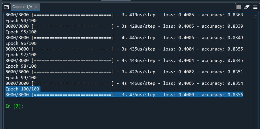

We have Accuracy Score of 83.5% remember that. Now let’s

请记住，我们的准确率是83.5％。现在让我们

Grid Search the batch_size and epochs then followed by
网格搜索batch_size和纪元，然后是
Grid Search Optimizer
网格搜索优化器
Grid Search Learning Rate and Momentum
网格搜索学习率和动量
Network Weight Initialization
网络权重初始化
Neuron Activation
神经元激活
Tune Dropout Regularization
调音辍学正则化
Tune Drop out Regularization
调出辍学正规化
Tune Number of Neurons
神经元调数

#scikit-learn to grid search the batch size and epochsimport numpy
from sklearn.model_selection import GridSearchCV
from keras.models import Sequential
from keras.layers import Dense
from keras.wrappers.scikit_learn import KerasClassifier#Function to create model, required for KerasClassifier
def create_model():
model=Sequential()
model.add(Dense(units = 6, kernel_initializer='uniform',activation = 'relu',input_dim = 11))
model.add(Dense(units = 6, kernel_initializer='uniform',activation = 'relu'))
model.add(Dense(units = 1, kernel_initializer = 'uniform', activation = 'sigmoid'))#compile model
model.compile(optimizer = 'adam',loss = 'binary_crossentropy', metrics = ['accuracy'])return model#Importing the libraries
import numpy as np
import pandas as pd#Importing the dataset
dataset = pd.read_csv('Churn_Modelling.csv')X = dataset.iloc[:, 3:13].values
y = dataset.iloc[:, 13].values#Encoding categorical data
from sklearn.preprocessing import LabelEncoder, OneHotEncoder
from sklearn.compose import ColumnTransformer#country column
ct = ColumnTransformer([("Country", OneHotEncoder(), [1])], remainder = 'passthrough')X = ct.fit_transform(X)
#to avoid dummy variable trap
X = X[:, 1:]#Male/Female
labelencoder_X = LabelEncoder()
X[:, 3] = labelencoder_X.fit_transform(X[:, 3])#Splitting the dataset into the Training set and Test set
from sklearn.model_selection import train_test_split
X_train, X_test, y_train, y_test = train_test_split(X, y, test_size = 0.2, random_state = 0)#Feature Scaling
from sklearn.preprocessing import StandardScaler
sc = StandardScaler()
X_train = sc.fit_transform(X_train)
X_test = sc.transform(X_test)

Till here it’s the our regular data pre-processing step, now let’s define parameter list for batch size and epochs

到此为止，这是我们常规的数据预处理步骤，现在让我们定义批次大小和时期的参数列表

model = KerasClassifier(build_fn=create_model, verbose=1)#define the grid search parameters
batch_size = [10, 20, 40]
epochs = [10, 50,100,200]
param_grid = dict(batch_size=batch_size, epochs=epochs)
grid = GridSearchCV(estimator=model, param_grid=param_grid,cv=3)
grid_result = grid.fit(X_train, y_train)

Here we have first bind the list of parameters as dict ‘dictionary’ in param_grid then define our model in estimator and the parameter list in param_grid with cross validation cv = 3, means it will test 3 times and will give u the average results of 3 iterations.

在这里，我们首先在param_grid中将参数列表绑定为dict'dictionary'，然后在estimator中定义我们的模型，并在param_grid中使用交叉验证cv = 3定义参数列表，这意味着它将测试3次，并将得到3的平均结果迭代。

Finally we will summarize the results.

最后，我们将总结结果。

#summarize results
print("Best: %f using %s" % (grid_result.best_score_, grid_result.best_params_))means = grid_result.cv_results_['mean_test_score']
stds = grid_result.cv_results_['std_test_score']params = grid_result.cv_results_['params']
for mean, stdev, param in zip(means, stds, params):
print("%f (%f) with: %r" % (mean, stdev, param))

Let me put all the pieces together.

让我把所有的东西放在一起。

#tune Batch_size and epoch
#Use scikit-learn to grid search the batch size and epochs
import numpy
from sklearn.model_selection import GridSearchCV
from keras.models import Sequential
from keras.layers import Dense
from keras.wrappers.scikit_learn import KerasClassifier#Function to create model, required for KerasClassifier
def create_model():
    model=Sequential()
    model.add(Dense(units = 6, kernel_initializer='uniform',activation = 'relu',input_dim = 11))
    model.add(Dense(units = 6, kernel_initializer='uniform',activation = 'relu'))
    model.add(Dense(units = 1, kernel_initializer = 'uniform', activation = 'sigmoid'))
    #compile model
    model.compile(optimizer = 'adam',loss = 'binary_crossentropy', metrics = ['accuracy'])
    
    return model#Importing the libraries
import numpy as np
import matplotlib.pyplot as plt
import pandas as pd#Importing the dataset
dataset = pd.read_csv('Churn_Modelling.csv')
X = dataset.iloc[:, 3:13].values
y = dataset.iloc[:, 13].values#Encoding categorical data
from sklearn.preprocessing import LabelEncoder, OneHotEncoder
from sklearn.compose import ColumnTransformer#country column
ct = ColumnTransformer([("Country", OneHotEncoder(), [1])], remainder = 'passthrough')
X = ct.fit_transform(X)
#to avoid dummy variable trap
X = X[:, 1:]#Male/Female
labelencoder_X = LabelEncoder()
X[:, 3] = labelencoder_X.fit_transform(X[:, 3])#Splitting the dataset into the Training set and Test set
from sklearn.model_selection import train_test_split
X_train, X_test, y_train, y_test = train_test_split(X, y, test_size = 0.2, random_state = 0)#Feature Scaling
from sklearn.preprocessing import StandardScaler
sc = StandardScaler()
X_train = sc.fit_transform(X_train)
X_test = sc.transform(X_test)######################################################3#create model
model = KerasClassifier(build_fn=create_model, verbose=1)#define the grid search parameters
batch_size = [10, 20, 40]
epochs = [10, 50,100,200]
param_grid = dict(batch_size=batch_size, epochs=epochs)
grid = GridSearchCV(estimator=model, param_grid=param_grid,cv=3)grid_result = grid.fit(X_train, y_train)#summarize results
print("Best: %f using %s" % (grid_result.best_score_, grid_result.best_params_))means = grid_result.cv_results_['mean_test_score']
stds = grid_result.cv_results_['std_test_score']params = grid_result.cv_results_['params']
for mean, stdev, param in zip(means, stds, params):
    print("%f (%f) with: %r" % (mean, stdev, param))

We will have Output Best results as Epoch = 210, batch_size = 10

我们将获得最佳输出结果，因为时间= 210，batch_size = 10

Alright we have our best optimal epoch and batch_size settings that we need to put in our model to increase our model accuracy. Let’s redo our model with these settings and see if it improves or not.

好了，我们有最好的最佳纪元和batch_size设置，我们需要将它们放入模型中以提高模型的准确性。让我们使用这些设置重做我们的模型，看看它是否有所改善。

#Importing the libraries
import numpy as np
import matplotlib.pyplot as plt
import pandas as pd#Importing the dataset
dataset = pd.read_csv('Churn_Modelling.csv')
X = dataset.iloc[:, 3:13].values
y = dataset.iloc[:, 13].values#Encoding categorical data
from sklearn.preprocessing import LabelEncoder, OneHotEncoder
from sklearn.compose import ColumnTransformer#country column
ct = ColumnTransformer([("Country", OneHotEncoder(), [1])], remainder = 'passthrough')
X = ct.fit_transform(X)
#to avoid dummy variable trap
X = X[:, 1:]#Male/Female
labelencoder_X = LabelEncoder()
X[:, 3] = labelencoder_X.fit_transform(X[:, 3])#Splitting the dataset into the Training set and Test set
from sklearn.model_selection import train_test_split
X_train, X_test, y_train, y_test = train_test_split(X, y, test_size = 0.2, random_state = 0)#Feature Scaling
from sklearn.preprocessing import StandardScaler
sc = StandardScaler()
X_train = sc.fit_transform(X_train)
X_test = sc.transform(X_test)#Part 2 - Now let's make the ANN!#Importing the Keras libraries and packages
import keras
from keras.models import Sequential
from keras.layers import Dense#Initialising the ANN
classifier = Sequential()#Adding the input layer and the first hidden layer
classifier.add(Dense(units = 6, kernel_initializer = 'uniform', activation = 'relu', input_dim = 11))#Adding the second hidden layer
classifier.add(Dense(units = 6, kernel_initializer = 'uniform', activation = 'relu'))#Adding the output layer
classifier.add(Dense(units = 1, kernel_initializer = 'uniform', activation = 'sigmoid'))#Compiling the ANN
classifier.compile(optimizer = 'adam', loss = 'binary_crossentropy', metrics = ['accuracy'])#Fitting the ANN to the Training set
classifier.fit(X_train, y_train, batch_size = 10, epochs = 210)#Part 3 - Making the predictions and evaluating the model#Predicting the Test set results
y_pred = classifier.predict(X_test)
y_pred = (y_pred > 0.5)#Making the Confusion Matrix
from sklearn.metrics import confusion_matrix
cm = confusion_matrix(y_test, y_pred)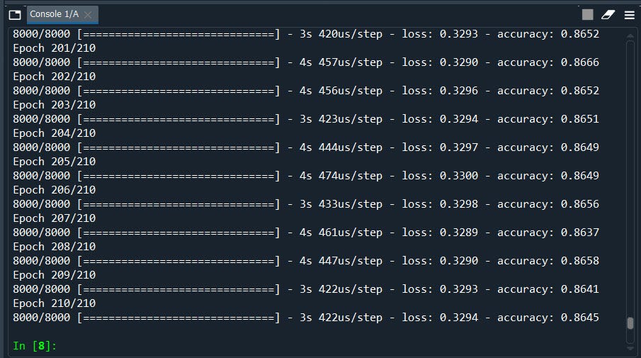

Nice! we have improved our model from 83% to 86%

真好！我们已将模型从83％改进为86％

2.) Next we will use Grid Search to find the best optimizer

2.)接下来，我们将使用网格搜索找到最佳的优化器

Optimizer in brief: optimizer are the algorithms or the methods that is used to calculate weights in order to reduce the losses. I guess you have already heard of Stochastic Gradient Descent and how it works. In layman’s term weights are the optimal values(calculations) that has low loss, in turn high accuracy.

简而言之，优化器：优化器是用于计算权重以减少损失的算法或方法。我想您已经听说过随机梯度下降及其工作原理。用外行术语来说，权重是具有低损耗，进而具有高准确性的最佳值(计算)。

The syntax are almost similar only we need few modification

语法几乎类似，只需要很少的修改

#Function to create model, required for KerasClassifierdef create_model(optimizer='adam'):model=Sequential()
model.add(Dense(units = 6, kernel_initializer='uniform',activation = 'relu',input_dim = 11))
model.add(Dense(units = 6, kernel_initializer='uniform',activation = 'relu'))
model.add(Dense(units = 1, kernel_initializer = 'uniform', activation = 'sigmoid'))#compile model
model.compile(optimizer = optimizer,loss = 'binary_crossentropy', metrics = ['accuracy'])return model########################################################define the grid search parameters
optimizer = ['SGD', 'RMSprop', 'Adagrad', 'Adadelta', 'Adam', 'Adamax', 'Nadam']
param_grid = dict(optimizer=optimizer)
grid = GridSearchCV(estimator=model, param_grid=param_grid, cv=3)grid_result = grid.fit(X_train, y_train)

Done! Let’s put all of the pieces together, run the code and see what we got!

做完了！让我们将所有部分放在一起，运行代码，看看我们得到了什么！

# Use scikit-learn to grid search the optimizer
import numpy
from sklearn.model_selection import GridSearchCV
from keras.models import Sequential
from keras.layers import Dense
from keras.wrappers.scikit_learn import KerasClassifier# Function to create model, required for KerasClassifier
def create_model(optimizer='adam'):
    model=Sequential()
    model.add(Dense(units = 6, kernel_initializer='uniform',activation = 'relu',input_dim = 11))
    model.add(Dense(units = 6, kernel_initializer='uniform',activation = 'relu'))
    model.add(Dense(units = 1, kernel_initializer = 'uniform', activation = 'sigmoid'))
    #compile model
    model.compile(optimizer = optimizer,loss = 'binary_crossentropy', metrics = ['accuracy'])
    
    return model#Importing the libraries
import numpy as np
import matplotlib.pyplot as plt
import pandas as pd#Importing the dataset
dataset = pd.read_csv('Churn_Modelling.csv')
X = dataset.iloc[:, 3:13].values
y = dataset.iloc[:, 13].values#Encoding categorical data
from sklearn.preprocessing import LabelEncoder, OneHotEncoder
from sklearn.compose import ColumnTransformer#country column
ct = ColumnTransformer([("Country", OneHotEncoder(), [1])], remainder = 'passthrough')
X = ct.fit_transform(X)
#to avoid dummy variable trap
X = X[:, 1:]#Male/Female
labelencoder_X = LabelEncoder()
X[:, 3] = labelencoder_X.fit_transform(X[:, 3])#Splitting the dataset into the Training set and Test set
from sklearn.model_selection import train_test_split
X_train, X_test, y_train, y_test = train_test_split(X, y, test_size = 0.2, random_state = 0)#Feature Scaling
from sklearn.preprocessing import StandardScaler
sc = StandardScaler()
X_train = sc.fit_transform(X_train)
X_test = sc.transform(X_test)#############################################################
#create model
model = KerasClassifier(build_fn=create_model, epochs=200, batch_size=10, verbose=1)#define the grid search parameters
optimizer = ['SGD', 'RMSprop', 'Adagrad', 'Adadelta', 'Adam', 'Adamax', 'Nadam']
param_grid = dict(optimizer=optimizer)grid = GridSearchCV(estimator=model, param_grid=param_grid, cv=3)
grid_result = grid.fit(X_train, y_train)#summarize results
print("Best: %f using %s" % (grid_result.best_score_, grid_result.best_params_))means = grid_result.cv_results_['mean_test_score']
stds = grid_result.cv_results_['std_test_score']params = grid_result.cv_results_['params']
for mean, stdev, param in zip(means, stds, params):
    print("%f (%f) with: %r" % (mean, stdev, param))

We will have Output Best results as optimizer = SGD ~ Stochastic Gradient Descent.

当优化程序= SGD〜随机梯度下降时，我们将获得最佳输出结果。

The results may vary depending on seed value as well as cross validation cv value. It takes time to get the output. Therefore i decided to write the output from my records rather than using screenshot.

结果可能会因种子值以及交叉验证CV值而异。获取输出需要时间。因此，我决定从记录中写入输出，而不是使用屏幕截图。

Now let’s use the optimizer as ‘SGD’ and see how much it improves. Generally ‘adam’ is the commonly used but believed to be optimized version of all. But in few cases other optimizer out performs ‘adam’ such as these one.

现在，让我们将优化器用作“ SGD”，然后看看它可以改进多少。通常， “ adam”是常用的，但被认为是所有版本的优化版本。但是在少数情况下，其他优化器也会执行诸如此类的“调整” 。

#Importing the libraries
import numpy as np
import matplotlib.pyplot as plt
import pandas as pd#Importing the dataset
dataset = pd.read_csv('Churn_Modelling.csv')
X = dataset.iloc[:, 3:13].values
y = dataset.iloc[:, 13].values#Encoding categorical data
from sklearn.preprocessing import LabelEncoder, OneHotEncoder
from sklearn.compose import ColumnTransformer#country column
ct = ColumnTransformer([("Country", OneHotEncoder(), [1])], remainder = 'passthrough')
X = ct.fit_transform(X)
#to avoid dummy variable trap
X = X[:, 1:]#Male/Female
labelencoder_X = LabelEncoder()
X[:, 3] = labelencoder_X.fit_transform(X[:, 3])#Splitting the dataset into the Training set and Test set
from sklearn.model_selection import train_test_split
X_train, X_test, y_train, y_test = train_test_split(X, y, test_size = 0.2, random_state = 0)#Feature Scaling
from sklearn.preprocessing import StandardScaler
sc = StandardScaler()
X_train = sc.fit_transform(X_train)
X_test = sc.transform(X_test)#Importing the Keras libraries and packages
import keras
from keras.models import Sequential
from keras.layers import Dense#Initialising the ANN
classifier = Sequential()#Adding the input layer and the first hidden layer
classifier.add(Dense(units = 6, kernel_initializer = 'uniform', activation = 'relu', input_dim = 11))#Adding the second hidden layer
classifier.add(Dense(units = 6, kernel_initializer = 'uniform', activation = 'relu'))# Adding the output layer
classifier.add(Dense(units = 1, kernel_initializer = 'uniform', activation = 'sigmoid'))#Compiling the ANN
classifier.compile(optimizer = 'SGD', loss = 'binary_crossentropy', metrics = ['accuracy'])#Fitting the ANN to the Training set
classifier.fit(X_train, y_train, batch_size = 10, epochs = 100)#Part 3 - Making the predictions and evaluating the model#Predicting the Test set results
y_pred = classifier.predict(X_test)
y_pred = (y_pred > 0.5)#Making the Confusion Matrix
from sklearn.metrics import confusion_matrix
cm = confusion_matrix(y_test, y_pred)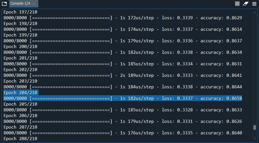

Well we have slightly improved our model with the SGD optimizer early at 204 epoch, probably because of my seed number.

好吧，在204年代初，我们使用SGD优化器对模型进行了稍微改进，这可能是因为我的种子数。

Next we have Learning rate and the momentum.

接下来，我们将了解学习率和发展势头。

3.) Learning Rate and momentum

3.)学习率和动力

Learning rate in brief: The amount of rate that the weights are updated during training is referred as the step size or the “learning rate.” Learning rate measures how much the current situation affects the next step, while momentum measures how much past steps affect the next step.

简短的学习率：训练期间权重更新的率的数量称为步长或“学习率”。 学习率衡量当前情况对下一步的影响，而动量则衡量过去的步骤对下一步的影响。

In simple words, it’s the number of steps that will be used to calculate the weights.

简而言之，就是用于计算权重的步骤数。

We will use the same template with few modifications for get the best learning rate and momentum.

我们将使用相同的模板，进行少量修改以获取最佳的学习速度和动力。

def create_model(learn_rate=0.01, momentum=0):model=Sequential()
model.add(Dense(units = 6, kernel_initializer='uniform',activation = 'relu',input_dim = 11))
model.add(Dense(units = 6, kernel_initializer='uniform',activation = 'relu'))
model.add(Dense(units = 1, kernel_initializer = 'uniform', activation = 'sigmoid'))
optimizer = SGD(lr=0.01,momentum = momentum)#compile model
model.compile(optimizer = optimizer,loss = 'binary_crossentropy', metrics = ['accuracy'])
return model##############################################3#define the grid search parameters
learn_rate = [0.001, 0.01, 0.1, 0.2, 0.3]
momentum = [0.0, 0.2, 0.4, 0.6, 0.8, 0.9]
param_grid = dict(learn_rate=learn_rate, momentum=momentum)grid = GridSearchCV(estimator=model, param_grid=param_grid, cv=3)

Let’s put all of this together and see what we got.

让我们将所有这些放在一起，看看我们得到了什么。

#Use scikit-learn to grid search the learning rate and momentum
import numpy
from sklearn.model_selection import GridSearchCV
from keras.models import Sequentialfrom keras.layers import Densefrom keras.wrappers.scikit_learn import KerasClassifier
from keras.optimizers import SGD#Function to create model, required for KerasClassifier
def create_model(learn_rate=0.01, momentum=0):model=Sequential()
model.add(Dense(units = 6, kernel_initializer='uniform',activation = 'relu',input_dim = 11))
model.add(Dense(units = 6, kernel_initializer='uniform',activation = 'relu'))
model.add(Dense(units = 1, kernel_initializer = 'uniform', activation = 'sigmoid'))
optimizer = SGD(lr=0.01,momentum = momentum)#compile model
model.compile(optimizer = optimizer,loss = 'binary_crossentropy', metrics = ['accuracy'])return model#Importing the libraries
import numpy as np
import matplotlib.pyplot as plt
import pandas as pd#Importing the dataset
dataset = pd.read_csv('Churn_Modelling.csv')
X = dataset.iloc[:, 3:13].values
y = dataset.iloc[:, 13].values#Encoding categorical data
from sklearn.preprocessing import LabelEncoder, OneHotEncoder
from sklearn.compose import ColumnTransformer#country column
ct = ColumnTransformer([("Country", OneHotEncoder(), [1])], remainder = 'passthrough')
X = ct.fit_transform(X)#to avoid dummy variable trap
X = X[:, 1:]#Male/Female
labelencoder_X = LabelEncoder()
X[:, 3] = labelencoder_X.fit_transform(X[:, 3])#Splitting the dataset into the Training set and Test set
from sklearn.model_selection import train_test_split
X_train, X_test, y_train, y_test = train_test_split(X, y, test_size = 0.2, random_state = 0)#Feature Scaling
from sklearn.preprocessing import StandardScalersc = StandardScaler()
X_train = sc.fit_transform(X_train)
X_test = sc.transform(X_test)##################################################create model
model = KerasClassifier(build_fn=create_model, epochs=210, batch_size=10, verbose=1)#define the grid search parameters
learn_rate = [0.001, 0.01, 0.1, 0.2, 0.3]
momentum = [0.0, 0.2, 0.4, 0.6, 0.8, 0.9]
param_grid = dict(learn_rate=learn_rate, momentum=momentum)grid = GridSearchCV(estimator=model, param_grid=param_grid, cv=3)
grid_result = grid.fit(X_train, y_train)#summarize results
print("Best: %f using %s" % (grid_result.best_score_, grid_result.best_params_))means = grid_result.cv_results_['mean_test_score']
stds = grid_result.cv_results_['std_test_score']
params = grid_result.cv_results_['params']
for mean, stdev, param in zip(means, stds, params):
print("%f (%f) with: %r" % (mean, stdev, param))

We will have a output of Best learning rate of 0.01 and a momentum of 0.5

我们的最佳学习率输出为0.01，动量为0.5

Now we can use these learning rate and momentum in our optimizer to improve our accuracy score.

现在，我们可以在优化器中使用这些学习率和动量来提高准确性得分。

Next we will move on to Kernel initializer.

接下来，我们将转到内核初始化程序。

4.) Kernel Initializer

4.)内核初始化

Kernel initializer is a fancy term for which statistical distribution or function to use for initialising the weights.

内核初始化程序是一个花哨的术语，其统计分布或函数用于初始化权重。

As usual we only need few modifications for kernel initializer

像往常一样，我们只需要对内核初始化程序进行少量修改

#Function to create model, required for KerasClassifier
def create_model(init_mode='uniform'):model=Sequential()
model.add(Dense(units = 6, kernel_initializer= init_mode, activation = 'relu',input_dim = 11))
model.add(Dense(units = 6, kernel_initializer='uniform',activation = 'relu'))
model.add(Dense(units = 1, kernel_initializer = 'uniform', activation = 'sigmoid'))#compile model
model.compile(optimizer = 'SGD',loss = 'binary_crossentropy', metrics = ['accuracy'])
return model############################################
#create model
model = KerasClassifier(build_fn=create_model, epochs=210, batch_size=10, verbose=1)#define the grid search parameters
init_mode = ['uniform', 'lecun_uniform', 'normal', 'zero', 'glorot_normal', 'glorot_uniform', 'he_normal', 'he_uniform']
param_grid = dict(init_mode=init_mode)
grid = GridSearchCV(estimator=model, param_grid=param_grid, cv=3)
grid_result = grid.fit(X_train, y_train)

Done! Let’s put all the pieces together and see which kernel initializer is the best.

做完了！让我们将所有内容放在一起，看看哪种内核初始化程序是最好的。

#Kernal Initializationimport numpy
from sklearn.model_selection import GridSearchCV
from keras.models import Sequential
from keras.layers import Dense
from keras.wrappers.scikit_learn import KerasClassifier
from keras.optimizers import SGD#Function to create model, required for KerasClassifier
def create_model(init_mode='uniform'):model=Sequential()
model.add(Dense(units = 6, kernel_initializer= init_mode, activation = 'relu',input_dim = 11))
model.add(Dense(units = 6, kernel_initializer='uniform',activation = 'relu'))
model.add(Dense(units = 1, kernel_initializer = 'uniform', activation = 'sigmoid'))#compile model
model.compile(optimizer = 'SGD',loss = 'binary_crossentropy', metrics = ['accuracy'])return model#Importing the libraries
import numpy as np
import matplotlib.pyplot as plt
import pandas as pd#Importing the dataset
dataset = pd.read_csv('Churn_Modelling.csv')
X = dataset.iloc[:, 3:13].values
y = dataset.iloc[:, 13].values#Encoding categorical data
from sklearn.preprocessing import LabelEncoder, OneHotEncoder
from sklearn.compose import ColumnTransformer#country column
ct = ColumnTransformer([("Country", OneHotEncoder(), [1])], remainder = 'passthrough')
X = ct.fit_transform(X)
#to avoid dummy variable trap
X = X[:, 1:]#Male/Female
labelencoder_X = LabelEncoder()
X[:, 3] = labelencoder_X.fit_transform(X[:, 3])#Splitting the dataset into the Training set and Test set
from sklearn.model_selection import train_test_split
X_train, X_test, y_train, y_test = train_test_split(X, y, test_size = 0.2, random_state = 0)#Feature Scalingfrom sklearn.preprocessing import StandardScaler
sc = StandardScaler()
X_train = sc.fit_transform(X_train)
X_test = sc.transform(X_test)#############################################create model
model = KerasClassifier(build_fn=create_model, epochs=210, batch_size=10, verbose=1)#define the grid search parameters
init_mode = ['uniform', 'lecun_uniform', 'normal', 'zero', 'glorot_normal', 'glorot_uniform', 'he_normal', 'he_uniform']
param_grid = dict(init_mode=init_mode)grid = GridSearchCV(estimator=model, param_grid=param_grid, cv=3)
grid_result = grid.fit(X_train, y_train)#summarize results
print("Best: %f using %s" % (grid_result.best_score_, grid_result.best_params_))means = grid_result.cv_results_['mean_test_score']
stds = grid_result.cv_results_['std_test_score']params = grid_result.cv_results_['params']
for mean, stdev, param in zip(means, stds, params):
print("%f (%f) with: %r" % (mean, stdev, param))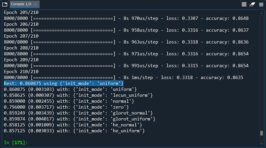

Well what got here….. The best average score is ‘uniform’ which we are already using.

好吧，这是什么…..最好的平均分数是我们已经在使用的“统一” 。

Next we have Neuron Activation.

接下来，我们进行神经元激活。

5.) Neuron activation is the parameter where we define the non-linearity function such as relu, sigmoid, leaky relu, softmax. I believe you are already aware of working of those functions. However the would like to mention the rule of thumb for the most commonly used activation functions

5. )神经元激活是我们定义非线性函数的参数，例如relu，Sigmoid，leaky relu，softmax。 我相信您已经意识到这些功能的工作。 但是，我们想提一下最常用的激活函数的经验法则

Relu is for non-linear data.

Relu用于非线性数据。

Sigmoid is if we want probability of 0 or 1, Yes or No in classification problem.

乙状结肠是我们是否希望分类问题中的概率为0或1，是或否。

Softmax is for when we perform multi-classification.

Softmax适用于我们执行多分类的情况。

To perform the Grid Search for neuron activation we will make few changes as shown below.

为了执行神经元激活的网格搜索，我们将进行如下所示的少量更改。

def create_model(activation='relu'):model=Sequential()
model.add(Dense(units = 6, kernel_initializer= 'uniform', activation = activation,input_dim = 11))
model.add(Dense(units = 6, kernel_initializer='uniform',activation = 'relu'))
model.add(Dense(units = 1, kernel_initializer = 'uniform', activation = 'sigmoid'))
#compile model
model.compile(optimizer = 'SGD',loss = 'binary_crossentropy', metrics = ['accuracy'])
return model################################################define the grid search parameters
activation = ['softmax', 'softplus', 'softsign', 'relu', 'tanh', 'sigmoid', 'hard_sigmoid', 'linear']
param_grid = dict(activation=activation)grid = GridSearchCV(estimator=model, param_grid=param_grid, cv=3)
grid_result = grid.fit(X_train, y_train)

Done! That’s it….. Let me put all of the pieces together, so that you can use it as template.

做完了！就这样.....让我将所有片段放在一起，以便您可以将其用作模板。

#grid search the Nuron activation function
import numpy
from sklearn.model_selection import GridSearchCV
from keras.models import Sequential
from keras.layers import Dense
from keras.wrappers.scikit_learn import KerasClassifierfrom keras.optimizers import SGD#Function to create model, required for KerasClassifier
def create_model(activation='relu'):
    model=Sequential()
    model.add(Dense(units = 6, kernel_initializer= 'uniform', activation = activation,input_dim = 11))
    model.add(Dense(units = 6, kernel_initializer='uniform',activation = 'relu'))
    model.add(Dense(units = 1, kernel_initializer = 'uniform', activation = 'sigmoid'))
    #compile model
    model.compile(optimizer = 'SGD',loss = 'binary_crossentropy', metrics = ['accuracy'])
    
    return model#Importing the libraries
import numpy as np
import matplotlib.pyplot as plt
import pandas as pd#Importing the dataset
dataset = pd.read_csv('Churn_Modelling.csv')
X = dataset.iloc[:, 3:13].values
y = dataset.iloc[:, 13].values# Encoding categorical data
from sklearn.preprocessing import LabelEncoder, OneHotEncoder
from sklearn.compose import ColumnTransformer#country column
ct = ColumnTransformer([("Country", OneHotEncoder(), [1])], remainder = 'passthrough')
X = ct.fit_transform(X)
#to avoid dummy variable trap
X = X[:, 1:]# Male/Female
labelencoder_X = LabelEncoder()
X[:, 3] = labelencoder_X.fit_transform(X[:, 3])# Splitting the dataset into the Training set and Test set
from sklearn.model_selection import train_test_split
X_train, X_test, y_train, y_test = train_test_split(X, y, test_size = 0.2, random_state = 0)# Feature Scaling
from sklearn.preprocessing import StandardScaler
sc = StandardScaler()
X_train = sc.fit_transform(X_train)
X_test = sc.transform(X_test)############################################
# create model
model = KerasClassifier(build_fn=create_model, epochs=210, batch_size=10, verbose=1)# define the grid search parameters
activation = ['softmax', 'softplus', 'softsign', 'relu', 'tanh', 'sigmoid', 'hard_sigmoid', 'linear']
param_grid = dict(activation=activation)grid = GridSearchCV(estimator=model, param_grid=param_grid, cv=3)
grid_result = grid.fit(X_train, y_train)#summarize results
print("Best: %f using %s" % (grid_result.best_score_, grid_result.best_params_))means = grid_result.cv_results_['mean_test_score']
stds = grid_result.cv_results_['std_test_score']params = grid_result.cv_results_['params']
for mean, stdev, param in zip(means, stds, params):
    print("%f (%f) with: %r" % (mean, stdev, param))

Well we got the best activation as ‘tanh’ for this example. Now if we put activation as ‘tanh’ it should increase the accuracy.

好吧，在此示例中，我们以“ tanh”获得了最佳激活。现在，如果我们将激活设置为“ tanh”，它将提高准确性。

# Importing the libraries
import numpy as np
import matplotlib.pyplot as plt
import pandas as pd#Importing the datasetdataset = pd.read_csv('Churn_Modelling.csv')
X = dataset.iloc[:, 3:13].values
y = dataset.iloc[:, 13].values#Encoding categorical data
from sklearn.preprocessing import LabelEncoder, OneHotEncoder
from sklearn.compose import ColumnTransformer#country column
ct = ColumnTransformer([("Country", OneHotEncoder(), [1])], remainder = 'passthrough')X = ct.fit_transform(X)
#to avoid dummy variable trap
X = X[:, 1:]#Male/Female
labelencoder_X = LabelEncoder()
X[:, 3] = labelencoder_X.fit_transform(X[:, 3])#Splitting the dataset into the Training set and Test set
from sklearn.model_selection import train_test_split
X_train, X_test, y_train, y_test = train_test_split(X, y, test_size = 0.2, random_state = 0)#Feature Scaling
from sklearn.preprocessing import StandardScaler
sc = StandardScaler()
X_train = sc.fit_transform(X_train)
X_test = sc.transform(X_test)#Importing the Keras libraries and packages
import keras
from keras.models import Sequential
from keras.layers import Dense#Initialising the ANN
classifier = Sequential()#Adding the input layer and the first hidden layer
classifier.add(Dense(units = 6, kernel_initializer = 'uniform', activation = 'tanh', input_dim = 11))#Adding the second hidden layer
classifier.add(Dense(units = 6, kernel_initializer = 'uniform', activation = 'relu'))#Adding the output layer
classifier.add(Dense(units = 1, kernel_initializer = 'uniform', activation = 'sigmoid'))#Compiling the ANN
classifier.compile(optimizer = 'adam', loss = 'binary_crossentropy', metrics = ['accuracy'])#Fitting the ANN to the Training set
classifier.fit(X_train, y_train, batch_size = 10, epochs = 210)#Part 3 - Making the predictions and evaluating the model#Predicting the Test set results
y_pred = classifier.predict(X_test)
y_pred = (y_pred > 0.5)#Making the Confusion Matrix
from sklearn.metrics import confusion_matrix
cm = confusion_matrix(y_test, y_pred)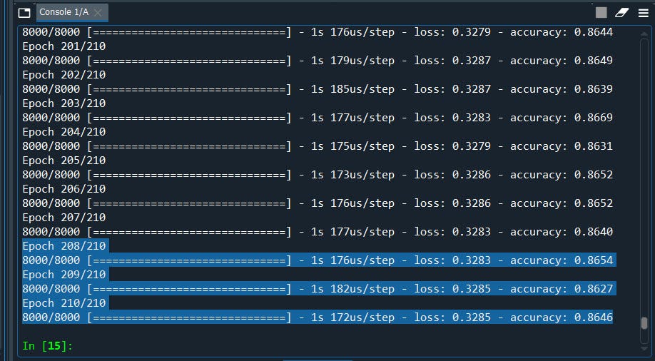

yes, it did by few decimals.

是的，它只有几位小数。

Next we have Grid Search for Drop Out Regularization

接下来，我们进行网格搜索以进行辍学正则化

Drop out is a technique used to prevent a model from overfitting. It is applied between the hidden layers and between the last hidden layer. In simple words the term ‘dropout’ refers to dropping out units (Both hidden and visible) in a neural network

退出是用于防止模型过度拟合的技术。它应用于隐藏层之间以及最后一个隐藏层之间。简而言之，术语“退出”是指在神经网络中退出单位(隐藏的和可见的)

Imagine that if neurons are randomly dropped out of the network during training, that other neurons will have to step in and handle the representation required to make predictions for the missing neurons. This is believed to result in multiple independent internal representations being learned by the network.

想象一下，如果在训练过程中神经元随机掉出网络，那么其他神经元将不得不介入并处理预测缺失神经元所需的表示。据信这导致网络学习到多个独立的内部表示。

The effect is that the network becomes less sensitive to the specific weights of neurons. This in turn results in a network that is capable of better generalization and is less likely to overfit the training data.

效果是网络对神经元的特定权重变得不那么敏感。反过来，这会导致网络具有更好的泛化能力，并且不太可能过度拟合训练数据。

Weight constraints also provide an approach to reduce the overfitting of a deep learning neural network model on the training data to improve the performance of the model for new data.

权重约束还提供了一种方法，可以减少深度学习神经网络模型对训练数据的过度拟合，从而改善新数据模型的性能。

A suite of different vector norms can be used as constraints, provided as classes in the keras.constraints module. They are:

一组不同的矢量规范可以用作约束，在keras.constraints模块中作为类提供。他们是：

· Maximum norm (max_norm), to force weights to have a magnitude at or below a given limit.

· 最大范数 ( max_norm )，以强制权重达到或小于给定限制的大小。

· Non-negative norm (non_neg), to force weights to have a positive magnitude.

· 非负范数 ( non_neg )，强制权重具有正值。

· Unit norm (unit_norm), to force weights to have a magnitude of 1.0.

· 单位范数 ( unit_norm )，强制权重的大小为1.0。

· Min-Max norm (min_max_norm), to force weights to have a magnitude between a range.

· Min-Max范数 ( min_max_norm )，以强制权重在一个范围内。

Now lets see how can we apply Grid Search for Dropout and Weight Constraints.

现在，让我们看看如何将网格搜索应用于辍学和权重约束。

from keras.constraints import maxnorm
from keras.layers import Dropout#Function to create model, required for KerasClassifier
def create_model(dropout_rate=0.0, weight_constraint=0):
    model=Sequential()
    model.add(Dense(units = 6, kernel_initializer= 'uniform', activation = 'tanh',kernel_constraint=maxnorm(weight_constraint),input_dim = 11))
    model.add(Dense(units = 6, kernel_initializer='uniform',activation = 'relu'))
    model.add(Dropout(dropout_rate))
    model.add(Dense(units = 1, kernel_initializer = 'uniform', activation = 'sigmoid'))
    #compile model
    model.compile(optimizer = 'SGD',loss = 'binary_crossentropy', metrics = ['accuracy'])
    
    return model################################################define the grid search parameters
weight_constraint = [1, 2, 3, 4, 5]
dropout_rate = [0.0, 0.1, 0.2, 0.3, 0.4, 0.5, 0.6, 0.7, 0.8, 0.9]
param_grid = dict(dropout_rate=dropout_rate, weight_constraint=weight_constraint)

Alright the whole code looks the same with few modifications. let me put all the pieces together so that you can use this as a template

好了，整个代码看起来几乎没有什么修改。让我将所有部分放在一起，以便您可以将其用作模板

#grid search the Dropout Regularization
import numpy
from sklearn.model_selection import GridSearchCV
from keras.models import Sequential
from keras.layers import Dense
from keras.wrappers.scikit_learn import KerasClassifierfrom keras.optimizers import SGD
from keras.constraints import maxnorm
from keras.layers import Dropout#Function to create model, required for KerasClassifier
def create_model(dropout_rate=0.0, weight_constraint=0):
    model=Sequential()
    model.add(Dense(units = 6, kernel_initializer= 'uniform', activation = 'tanh',kernel_constraint=maxnorm(weight_constraint),input_dim = 11))
    model.add(Dense(units = 6, kernel_initializer='uniform',activation = 'relu'))
    model.add(Dropout(dropout_rate))
    model.add(Dense(units = 1, kernel_initializer = 'uniform', activation = 'sigmoid'))
    #compile model
    model.compile(optimizer = 'SGD',loss = 'binary_crossentropy', metrics = ['accuracy'])
    
    return model#Importing the libraries
import numpy as np
import pandas as pd#Importing the dataset
dataset = pd.read_csv('Churn_Modelling.csv')
X = dataset.iloc[:, 3:13].values
y = dataset.iloc[:, 13].values#Encoding categorical data
from sklearn.preprocessing import LabelEncoder, OneHotEncoder
from sklearn.compose import ColumnTransformer#country column
ct = ColumnTransformer([("Country", OneHotEncoder(), [1])], remainder = 'passthrough')
X = ct.fit_transform(X)
#to avoid dummy variable trap
X = X[:, 1:]#Male/Female
labelencoder_X = LabelEncoder()
X[:, 3] = labelencoder_X.fit_transform(X[:, 3])#Splitting the dataset into the Training set and Test set
from sklearn.model_selection import train_test_split
X_train, X_test, y_train, y_test = train_test_split(X, y, test_size = 0.2, random_state = 0)#Feature Scaling
from sklearn.preprocessing import StandardScaler
sc = StandardScaler()
X_train = sc.fit_transform(X_train)
X_test = sc.transform(X_test)############################################
#create model
model = KerasClassifier(build_fn=create_model, epochs=210, batch_size=10, verbose=1)#define the grid search parameters
weight_constraint = [1, 2, 3, 4, 5]
dropout_rate = [0.0, 0.1, 0.2, 0.3, 0.4, 0.5, 0.6, 0.7, 0.8, 0.9]
param_grid = dict(dropout_rate=dropout_rate, weight_constraint=weight_constraint)grid = GridSearchCV(estimator=model, param_grid=param_grid, cv=3)grid_result = grid.fit(X_train, y_train)#summarize results
print("Best: %f using %s" % (grid_result.best_score_, grid_result.best_params_))means = grid_result.cv_results_['mean_test_score']
stds = grid_result.cv_results_['std_test_score']params = grid_result.cv_results_['params']
for mean, stdev, param in zip(means, stds, params):
    print("%f (%f) with: %r" % (mean, stdev, param))

Finally we are into the last one Grid Search for the Best Optimal number of neurons.

最后，我们进入了最后一个网格搜索，以寻找最佳最佳神经元数。

7.) Grid Search for the Optimal Number of Neurons

7.)网格搜索神经元的最佳数量

As we know neuron takes one or more inputs that are computed by values called “weights” and then passed to a non-linear function which is known as an activation function,

我们知道神经元接受一个或多个输入，这些输入由称为“权重”的值计算，然后传递给称为激活函数的非线性函数，

In general the rule of thumb to select the best number of neurons is to take half of the actual input i.e. input dimensions (n/2). However we can also use the grid search feature to find the best optimal number of neurons so that we can improve our model.

通常，选择最佳神经元数量的经验法则是采用实际输入的一半，即输入尺寸(n / 2)。但是，我们还可以使用网格搜索功能来找到最佳的神经元最佳数量，以便改进模型。

#Function to create model, required for KerasClassifierdef create_model(neurons=1):
model=Sequential()
model.add(Dense(units =neurons, kernel_initializer= 'uniform', activation = 'tanh',kernel_constraint=maxnorm(4),input_dim = 11))
model.add(Dense(units = 6, kernel_initializer='uniform',activation = 'relu'))
model.add(Dropout(0.2))
model.add(Dense(units = 1, kernel_initializer = 'uniform', activation = 'sigmoid'))#compile model
model.compile(optimizer = 'SGD',loss = 'binary_crossentropy', metrics = ['accuracy'])
return model############################################define the grid search parameters
neurons = [1, 5, 10, 15, 20, 25, 30]
param_grid = dict(neurons=neurons)
grid = GridSearchCV(estimator=model, param_grid=param_grid, cv=3)
grid_result = grid.fit(X_train, y_train)

Let’s put all of these together to use it as template.

让我们将所有这些放在一起以用作模板。

#grid search the Dropout Regularization
import numpy
from sklearn.model_selection import GridSearchCV
from keras.models import Sequential
from keras.layers import Dense
from keras.wrappers.scikit_learn import KerasClassifierfrom keras.optimizers import SGD
from keras.constraints import maxnorm
from keras.layers import Dropout# Function to create model, required for KerasClassifier
def create_model(neurons=1):
    model=Sequential()
    model.add(Dense(units =neurons, kernel_initializer= 'uniform', activation = 'tanh',kernel_constraint=maxnorm(4),input_dim = 11))
    model.add(Dense(units = 6, kernel_initializer='uniform',activation = 'relu'))
    model.add(Dropout(0.2))
    model.add(Dense(units = 1, kernel_initializer = 'uniform', activation = 'sigmoid'))
    #compile model
    model.compile(optimizer = 'SGD',loss = 'binary_crossentropy', metrics = ['accuracy'])
    
    return model# Importing the libraries
import numpy as np
import matplotlib.pyplot as plt
import pandas as pd# Importing the dataset
dataset = pd.read_csv('Churn_Modelling.csv')
X = dataset.iloc[:, 3:13].values
y = dataset.iloc[:, 13].values# Encoding categorical data
from sklearn.preprocessing import LabelEncoder, OneHotEncoder
from sklearn.compose import ColumnTransformer#country column
ct = ColumnTransformer([("Country", OneHotEncoder(), [1])], remainder = 'passthrough')
X = ct.fit_transform(X)
#to avoid dummy variable trap
X = X[:, 1:]# Male/Female
labelencoder_X = LabelEncoder()
X[:, 3] = labelencoder_X.fit_transform(X[:, 3])# Splitting the dataset into the Training set and Test set
from sklearn.model_selection import train_test_split
X_train, X_test, y_train, y_test = train_test_split(X, y, test_size = 0.2, random_state = 0)# Feature Scaling
from sklearn.preprocessing import StandardScaler
sc = StandardScaler()
X_train = sc.fit_transform(X_train)
X_test = sc.transform(X_test)############################################
# create model
model = KerasClassifier(build_fn=create_model, epochs=210, batch_size=10, verbose=1)# define the grid search parameters
neurons = [1, 5, 10, 15, 20, 25, 30]
param_grid = dict(neurons=neurons)grid = GridSearchCV(estimator=model, param_grid=param_grid, cv=3)grid_result = grid.fit(X_train, y_train)# summarize results
print("Best: %f using %s" % (grid_result.best_score_, grid_result.best_params_))means = grid_result.cv_results_['mean_test_score']
stds = grid_result.cv_results_['std_test_score']params = grid_result.cv_results_['params']
for mean, stdev, param in zip(means, stds, params):
    print("%f (%f) with: %r" % (mean, stdev, param))

We have our best score: 25 Let’s redo our model with 25 neurons

我们有我们最高的分数：25让我们用25个神经元重做模型

#Importing the libraries
import numpy as np
import matplotlib.pyplot as plt
import pandas as pdfrom keras.constraints import maxnorm
from keras.layers import Dropout#Importing the dataset
dataset = pd.read_csv('Churn_Modelling.csv')
X = dataset.iloc[:, 3:13].values
y = dataset.iloc[:, 13].values#Encoding categorical data
from sklearn.preprocessing import LabelEncoder, OneHotEncoder
from sklearn.compose import ColumnTransformer#country column
ct = ColumnTransformer([("Country", OneHotEncoder(), [1])], remainder = 'passthrough')
X = ct.fit_transform(X)
#to avoid dummy variable trap
X = X[:, 1:]#Male/Female
labelencoder_X = LabelEncoder()
X[:, 3] = labelencoder_X.fit_transform(X[:, 3])#Splitting the dataset into the Training set and Test set
from sklearn.model_selection import train_test_split
X_train, X_test, y_train, y_test = train_test_split(X, y, test_size = 0.2, random_state = 0)# Feature Scaling
from sklearn.preprocessing import StandardScaler
sc = StandardScaler()
X_train = sc.fit_transform(X_train)
X_test = sc.transform(X_test)# Part 2 - Now let's make the ANN!# Importing the Keras libraries and packages
import keras
from keras.models import Sequential
from keras.layers import Dense# Initialising the ANN
classifier = Sequential()#Adding the input layer and the first hidden layer
classifier.add(Dense(units = 25, kernel_initializer = 'uniform', activation = 'tanh', input_dim = 11))#Adding the second hidden layer
classifier.add(Dense(units = 6, kernel_initializer = 'uniform', activation = 'relu'))classifier.add(Dropout(0.2))#Adding the output layer
classifier.add(Dense(units = 1, kernel_initializer = 'uniform', activation = 'sigmoid'))#Compiling the ANN
classifier.compile(optimizer = 'adam', loss = 'binary_crossentropy', metrics = ['accuracy'])#Fitting the ANN to the Training set
classifier.fit(X_train, y_train, batch_size = 10, epochs = 210)#Part 3 - Making the predictions and evaluating the model#Predicting the Test set results
y_pred = classifier.predict(X_test)
y_pred = (y_pred > 0.5)#Making the Confusion Matrix
from sklearn.metrics import confusion_matrix
cm = confusion_matrix(y_test, y_pred)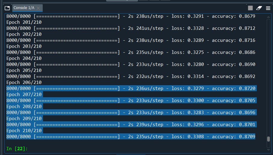

Nice. again we have improved our model from 86 to 87% and we have still have lot of room for improvement with few more tweaks.

真好再次，我们已将模型从86％改进到了87％，并且仍然有很大的改进空间，仅需进行少量调整即可。

Well it’s a long article, i tried my best to keep it as simple as possible keeping all the important concepts intact. I hope you enjoyed and able to use this Grid Search in your day to day deep learning methods.

好吧，这是一篇很长的文章，我尽力使它尽可能简单，以使所有重要概念完整无缺。希望您喜欢并能够在日常深度学习方法中使用此Grid Search。

My alternative internet presences, Facebook, Blogger, Linkedin, Medium, Instagram, ISSUU and my very own Data2Dimensions

我的其他互联网服务 ， Facebook ， Blogger ， Linkedin ， Medium， Instagram ， ISSUU和我自己的Data2Dimensions

Also available on Quora @ https://www.quora.com/profile/Bob-Rupak-Roy

也可以在Quora上找到 @ https://www.quora.com/profile/Bob-Rupak-Roy

Have a good day

祝你有美好的一天

Gain Access to Expert View — Subscribe to DDI Intel

获得访问专家视图的权限- 订阅DDI Intel

翻译自: https://medium.com/datadriveninvestor/grid-search-for-ml-deep-learning-models-260d07541b18

机器学习和深度学习的模型

weixin_26737625

关注

0
点赞
踩
1

收藏

觉得还不错? 一键收藏
0
评论
机器学习和深度学习的模型_机器学习和深度学习模型的网格搜索

机器学习和深度学习的模型Full guide to grid search on finding the best hyper parameters for our regular ml models to deep learning models 有关为常规ml模型到深度学习模型找到最佳超级参数的网格搜索的完整指南 Hi how are you doing, I hope its great....
复制链接

扫一扫